4  Gamma Regression

mindmap
  root((Regression 
  Analysis)
    Continuous <br/>Outcome Y
      {{Unbounded <br/>Outcome Y}}
        )Chapter 3: <br/>Ordinary <br/>Least Squares <br/>Regression(
          (Normal <br/>Outcome Y)
      {{Nonnegative <br/>Outcome Y}}
        )Chapter 4: <br/>Gamma Regression(
          (Gamma <br/>Outcome Y)
    Discrete <br/>Outcome Y

Figure 4.1: Regression analysis mind map depicting all modelling techniques explored so far in this book. Depending on the type of outcome \(Y\), these techniques are split into two large zones: discrete and continuous.

Learning Objectives

By the end of this chapter, you will be able to:

• Explain what Gamma regression is and when it is appropriate to use
• Recognize the types of problems suited for Gamma regression, especially those with positive, skewed outcomes
• Describe the Gamma distribution and how its shape is influenced by its parameters
• Understand the role of the link function, especially the log link, in Gamma regression
• Set up a Gamma regression model using a log link and interpret its coefficients in the context of the original variables
• Evaluate model fit using deviance residuals, spread patterns, and AIC

4.1 Introduction

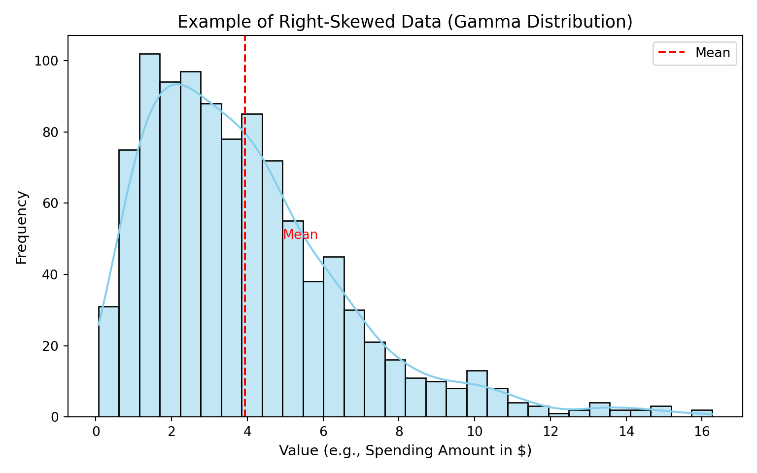
Some types of data are always positive and tend to have a few really large values. For example, imagine we are looking at how much people spend at a grocery store. Most people might spend a small to medium amount, but a few people might spend a lot more. This kind of data is not evenly spread out, and it does not look like a nice bell curve. Instead, it is skewed to the right, with a long tail of higher numbers.

In these situations, the usual type of regression (called ordinary least squares, or OLS) does not work very well. OLS assumes that the data is evenly spread out around the average and that big values and small values are equally likely. But when we have only positive numbers and some very big ones, we need a different approach.

This is where Gamma regression can help.

4.2 What is Gamma Regression

Gamma regression is a tool we use when the outcome we are trying to predict is always positive and can vary a lot. For example, we might want to predict:

• how long it takes for someone to complete a task
• how much money someone spends at a store
• the cost of a medical procedure

These types of outcomes are positive, continuous, and often right-skewed: most values are small or moderate, but a few can be extremely large. This uneven spread makes the data a poor fit for regular linear regression, which assumes that the outcomes are roughly symmetric and that the variability stays constant across all levels of the predictors.

Gamma regression is designed for situations like this. Instead of trying to fit a straight line with constant variance, it uses a model that:

• respects the fact that the outcome must be positive, and
• allows the variance to grow with the mean, which matches how many real-world cost or duration variables behave.

4.3 Understanding the Gamma Distribution

Gamma regression is built on something called the Gamma distribution. This distribution is used to describe values that are:

• always above zero
• and can have a long tail of larger values

What makes the Gamma distribution flexible is a number called the shape parameter. This controls how the data is spread out.

• When the shape is small (like 1), the distribution is very skewed. Most values are small, but a few are much larger.
• When the shape is larger (like 5 or 9), the curve becomes more balanced, though it still never includes negative numbers.

Let’s look at what this means visually:

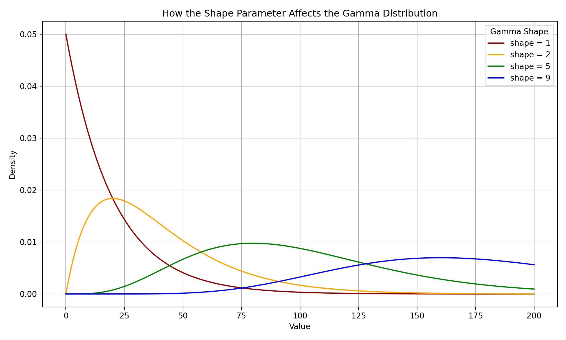
The plot above shows how the shape parameter changes the look of the Gamma distribution. It helps explain why Gamma regression is such a good match for skewed data. In the frequentist paradigm, we aim to find the Gamma distribution with the shape parameter that best fits the observed data.

4.4 How Gamma Regression Works

Now that we know what Gamma regression is and the kinds of problems it solves, let’s look at how it actually works.

The key idea is that Gamma regression doesn’t model the outcome values directly. Instead, it focuses on the average outcome and relates it to predictors in a way that respects the positive, skewed nature of the data.

To understand this, we need to take a step back and talk about a broader family of models called Generalized Linear Models, or GLMs. These are a flexible class of models that let us deal with many types of data, not just bell-shaped curves. GLMs allow us to model outcomes that are counts, proportions, or, as in our case, continuous and strictly positive. In this next section, we’ll break down what this means.

4.4.1 Generalized Linear Models

Definition of Generalized Linear Models

Generalized Linear Models (GLMs) are a powerful extension of linear regression. They allow us to model a wide variety of response variables beyond just those that follow a normal distribution. This makes GLMs especially useful in real-world situations where data often breaks the assumptions of ordinary least squares (OLS) regression.

Before we introduce the full GLM framework, let’s start with a simple example that shows why a standard linear model isn’t always appropriate. This will help motivate why we need a more general approach in the first place.

Problem with Linear Regression for Non-Normal Data

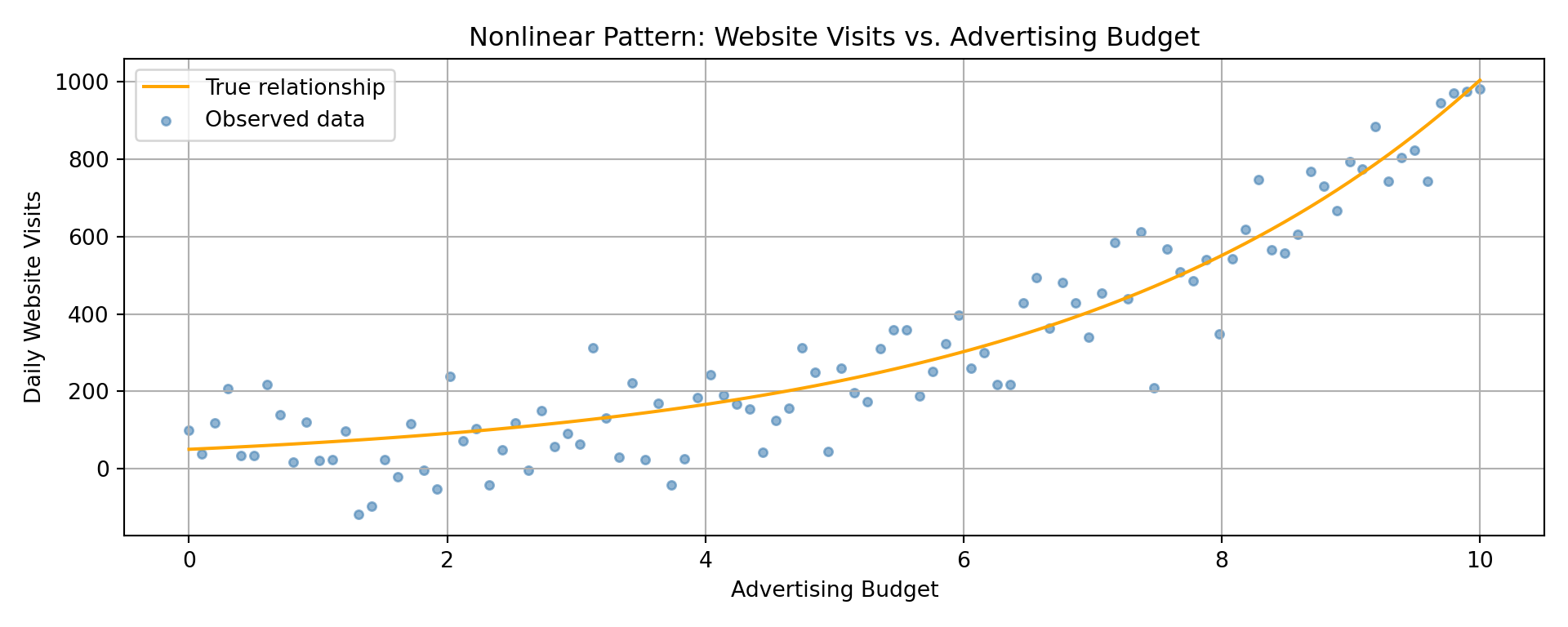
Suppose we want to model the number of daily website visits for a company, based on the company’s advertising budget. This outcome is:

• always positive
• right-skewed
• and often grows rapidly with budget

Let’s simulate this data:

Linear regression tries to fit a straight line through this data, but the result is clearly problematic.

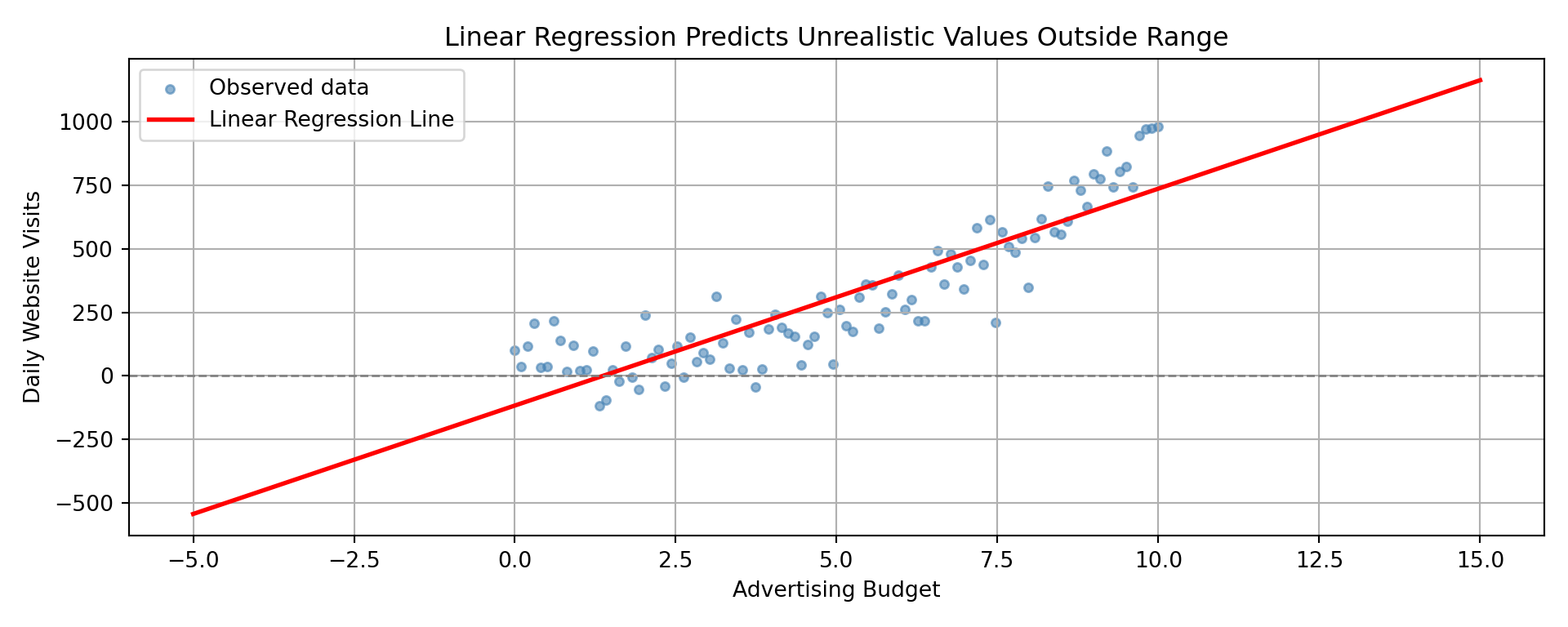
We run into several issues here:

• Predictions can be negative, which makes no sense for visit counts
• Predictions do not capture the multiplicative or curved nature of the relationship
• Variability grows with the mean, violating the constant variance assumption

These problems stem from assumptions built into OLS:

• The outcome is normally distributed
• The outcome has constant variance
• The relationship between predictors and outcome is linear

When those assumptions are broken, OLS can give misleading or invalid results.

What GLMs Do Differently

Despite these problems, linear regression has a big strength: it’s interpretable. The formula tells us exactly how the outcome changes with the predictor. But wouldn’t it be great if we could retain this interpretability while also accounting for the data’s quirks? That’s what Generalized Linear Models do.

The original linear regression formula looks like this:

\[ \mu = \beta_0 + \beta_1 x \]

As demonstrated above, this assumes \(\mu\) (the expected outcome) can take any real value, including negatives, and grows in a straight-line fashion, which just doesn’t make much sense given the data.

Now, imagine we make one small change, apply a log transformation to the mean:

\[ \log(\mu) = \beta_0 + \beta_1 x \]

This small adjustment makes a huge difference. Here’s how the fitted curve now looks with this small change:

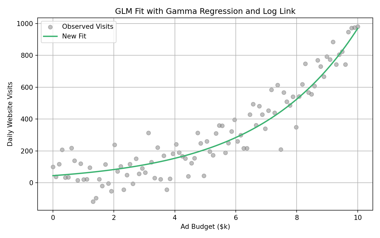
This new setup has several advantages:

• All predicted values of \(\mu\) are strictly positive
• The relationship between predictors and response is multiplicative, not additive
• The variance increases with the mean, which reflects how real-world data often behaves
• We still retain a straight-line interpretation, but now it’s on the log scale

What you have just witnessed is an example of Generalized Linear Model. It is a flexible extension of linear regression that allows you to model outcomes in a way that reflects how they are actually distributed, while also preserving the ability to interpret coefficients like in linear regression

The Three Components of GLM

Now that we have seen an example of a GLM, let’s properly introduce the components that make up a GLM. Every Generalized Linear Model (GLM) is built on the same three key components. This structure gives GLMs the flexibility to model many types of data while still being easy to interpret.

1. Random Component (Distribution of the Response)

This specifies how the response variable is distributed. In linear regression, the response is normally distributed. But GLMs allow for many other distributions, depending on what kind of data you are modeling.

Type of Data	Example Distribution
Continuous, symmetric	Normal
Count	Poisson
Proportion or binary	Binomial
Positive, skewed	Gamma

This is where the flexibility of GLMs comes from. You choose a distribution that matches your outcome.

2. Systematic Component (Linear Predictor)

This is the familiar part from linear regression. It is a linear combination of the predictors:

\[ \begin{align*} \eta &= \beta_0 + \beta_1 x_{1} + \beta_2 x_{2} + \cdots + \beta_p x_{p} \end{align*} \]

This linear predictor, often denoted by \(\eta\), is the foundation of the model. The link function (coming next) will connect this to the mean of the response variable.

3. Link Function (Connecting Predictors to the Mean)

The link function transforms the expected value of the response variable so that it can be modeled as a linear combination of predictors.

\[ \begin{align*} g(\mu) = \eta &= \beta_0 + \beta_1 x_{1} + \beta_2 x_{2} + \cdots + \beta_p x_{p} \end{align*} \]

Different distributions tend to pair with different link functions:

Distribution	Typical Link Function	Equation Example
Normal	Identity	\(\mu = \eta\)
Binomial	Logit	\(\log\left( \frac{\mu}{1 - \mu} \right) = \eta\)
Poisson	Log	\(\log(\mu) = \eta\)
Gamma	Log	\(\log(\mu) = \eta\)

The link function helps ensure that predictions stay within a valid range (e.g., probabilities stay between 0 and 1, counts stay positive, etc.).

Gamma Regression as a GLM

Now that we’ve introduced the components of a GLM, we can see that Gamma regression is not a completely new type of model. Instead, it is one specific case within the broader GLM framework. What makes Gamma regression special is that it is designed for situations where the outcome:

• is strictly positive
• tends to be right-skewed
• and often shows larger variance when the mean is higher

To make this concrete, let’s specify the three GLM components as they apply to Gamma regression:

1. Random Component (Gamma)

The response variable \(Y\) is assumed to follow a Gamma distribution, which is continuous, strictly positive, and right-skewed. The variance of \(Y\) increases with its mean, often expressed as: ​ \[ \operatorname{Var}(Y_i) = \phi \mu_i^2 \]

This makes Gamma regression a good match for data where larger expected values come with more uncertainty.

2. Systematic Component (Gamma)

Just like in linear regression, the predictors are combined linearly:

\[ \eta_i = \beta_0 + \beta_1 x_{i1} + \beta_2 x_{i2} + \cdots + \beta_p x_{ip} \]

This linear predictor \(\eta_i\) serves as the backbone of the model.

3. Link Function (Gamma)

To connect the predictors to the expected outcome \(\mu_i = \mathbb{E}(Y_i)\), Gamma regression uses the log link:

\[ \log(\mu_i) = \eta_i = \beta_0 + \beta_1 x_{i1} + \cdots + \beta_p x_{ip} \]

This ensures that:

• All predicted values of \(\mu_i\) are strictly positive
• The relationship between predictors and the mean is multiplicative, not additive
• We can interpret coefficients on the log scale, preserving interpretability

In other words, Gamma regression is just a GLM with a Gamma distribution and a log link. It does not model the outcome values directly. Instead, it focuses on the average outcome and relates it to predictors in a way that respects the positive, skewed nature of the data.

4.5 When to Use and Not Use Gamma Regression

With the core ideas of Gamma regression in place, we can now summarize the practical guidelines: the situations where Gamma regression is most effective, and the situations where it is not recommended.

When to Use and Not Use Gamma Regression

Gamma regression is powerful, but it isn’t a one-size-fits-all tool. It shines in some situations and breaks down in others. The checklist below can help you decide.

Use Gamma regression when:

• The outcome is continuous and strictly positive (e.g., insurance claim amounts, pollutant concentrations, operational spending).
• Observations are statistically independent.
• The distribution is right-skewed, where variance grows faster than the mean.
• You want to model the logarithm of the mean as a link function, which guarantees positive predictions.

Avoid Gamma regression when:

• The outcome includes zeros or negative values.
• The outcome is a count variable. In that case, consider alternatives like Classical Poisson, Negative Binomial, Zero-Inflated Poisson or Generalized Poisson.
• The variance increases at a constant rate with the mean, rather than at a faster rate (a sign another GLM family may be more appropriate).

4.6 Case Study: Modeling Web Server Performance

To demonstrate Gamma regression in action, we will walk through a case study using a toy dataset. This case study will help us understand what affects the response time of a web server. Specifically, how long it takes (in milliseconds) for the server to respond to a user’s request.

We will approach this case study using the data science workflow introduced in the first chapter. This ensures a structured approach to framing the problem, selecting a model, and building an interpretation based on the model’s results.

4.6.1 The Dataset

The toy dataset used to demonstrate captures various features of web requests across different servers and regions. Each row represents a single request and contains information about the server load, the number of users at the time, how complex the request was, and other related factors. Below is a summary of the variables:

Variable Name	Description
response_time_ms	The time it takes for the server to respond to a request (in milliseconds).
concurrent_users	Number of users on the server at the time of the request.
database_queries	Number of database queries triggered by the request.
cache_hit_rate	Percentage of data requests served from the cache (0 to 100).
server_load	Server CPU load at the time of the request (0 to 100).
time_of_day	Hour of the day when the request was made (0 = midnight, 23 = 11 PM).
day_of_week	Day of the week (e.g., Monday, Tuesday).
geographic_region	Geographic region where the request originated.
request_complexity	Categorical value describing request complexity: “Simple”, “Moderate”, or “Complex”.
cdn_usage	Whether a content delivery network was used (“Yes” or “No”).
memory_usage	Memory used on the server at the time of request (in percent).

Here’s a snapshot of the dataset:

response_time_ms	concurrent_users	database_queries	cache_hit_rate	server_load	time_of_day	day_of_week	geographic_region	request_complexity	cdn_usage	memory_usage
54.2	40	10	94.8	61.4	8	Saturday	North_America	Moderate	Yes	63.6
28.6	148	1	56.1	43.2	18	Thursday	North_America	Complex	Yes	25.5
50.2	195	14	94.6	67.0	1	Thursday	North_America	Complex	No	26.6
24.8	82	10	77.9	83.9	14	Monday	Africa	Simple	Yes	67.5
127.1	85	10	58.7	47.1	7	Thursday	South_America	Moderate	Yes	54.4

This dataset allows us to analyze performance differences in web servers under different conditions and determine what contributes to longer or shorter response times.

4.6.2 The Problem We’re Trying to Solve

In this case study, our goal is to analyze what drives differences in web server response times. Because response time is continuous, strictly positive, and often right-skewed, Gamma regression is a natural choice for modeling it.

The key question we aim to answer is:

Which server or request characteristics have the biggest influence on response time?

Answering this question requires more than just prediction. It requires understanding the relationships between server conditions, request features, and performance. In the next section, we’ll clarify our study design and show how Gamma regression supports this goal.

4.7 Study Design

In this case study, our goal is to understand what drives differences in web server response times. Because response time is continuous, strictly positive, and often right-skewed, Gamma regression is a natural modeling choice.

The broader objective is to uncover which server or request characteristics meaningfully influence response time. This requires more than simply forecasting future values. It requires understanding how different factors relate to average performance.

To make that purpose precise, we turn to the study design.

4.7.1 Inferential vs. Predictive Analysis

Following the data science workflow, our first step is to define the purpose of the analysis. As mentioned, our guiding question is:

Which server or request characteristics have the biggest influence on response time?

This question can be approached in two different ways, inferential or predictive, depending on what we want the analysis to achieve.

• Inferential analysis helps us understand and quantify how different variables affect the average outcome. For example: Does using a content delivery network (CDN) significantly reduce response time? How much slower are complex requests compared to simple ones?

• Predictive analysis, by contrast, is about making accurate forecasts. For instance: Can we predict the response time of a future request based on its characteristics?

Gamma regression can be used for either purpose, but our focus in this chapter is inferential, since our goal is to explain and quantify how different factors influence response time.

To that end, we will use Gamma regression to estimate how each feature affects the average response time while properly accounting for skewness in the outcome. This allows us to answer questions such as:

• How do concurrent users affect response time?
• Does request complexity lead to slower responses?
• What is the typical effect of CDN usage?
• How are server load and memory usage related to delays?

Our goal is not to build a black-box predictor, but to uncover which factors matter most and how they shape server performance, insights that can guide system tuning, policy decisions, and resource planning.

4.8 Data Collection and Wrangling

With our statistical question clearly defined, the next step is to make sure the data is suitable for analysis. Although we already have the dataset, it is useful to reflect on how this type of server performance data might have been collected. Understanding the data collection process helps us recognize potential limitations and prepare the data appropriately.

4.8.1 Data Collection

For a study like this, where we analyze server response times across different conditions, data could have been collected through several common methods:

• Server Logs: Most web servers automatically record detailed logs of every request. These logs typically include information like timestamps, request types, response time, server load, and geographic origin. This is a likely source for our dataset and provides reliable, machine-recorded data.

• Monitoring Tools: Infrastructure monitoring platforms such as New Relic, Datadog, or AWS CloudWatch can capture performance metrics in real time. These tools often collect a richer set of metrics, including CPU usage, memory usage, and cache hit rates.

• Simulated Load Testing: In controlled environments, engineers may run scripted performance tests to evaluate how different types of requests behave under varying traffic loads. While simulated data offers consistency, it may not reflect real-world user behavior.

Each data collection method has its own strengths and trade-offs:

• Server logs are objective but may lack high-level context (such as request complexity or user intent).
• Monitoring tools are detailed but might involve sampling or missing values due to downtime.
• Simulated tests offer control but may lack realism.

Regardless of how the data was collected, it’s important to check for common issues such as:

• Missing values in fields like server load or memory usage
  
• Incorrect or inconsistent formatting (e.g., “Yes” vs “yes” vs “TRUE”)
  
• Outliers in response time that may skew the results
  
• Categorical variables that need to be converted into a numerical format for modeling

All of these issues will be addressed in the next stage, data wrangling.

4.8.2 Data Wrangling

Once the data has been collected, the next step is to prepare it for modeling. Even reliable sources like server logs or monitoring tools produce raw data that needs cleaning before it can be used effectively.

For Gamma regression, data wrangling typically involves:

• Validating the response variable to ensure all values are strictly positive and meaningful.
• Transforming categorical variables (e.g., request complexity, geographic region) into numerical formats that the model can handle.
• Checking for missing values or extreme outliers that could bias results.
• Scaling or normalizing predictors if large differences in measurement units make interpretation difficult.

Let’s walk through how to apply these steps to our dataset.

1. Validating the Response Variable

Gamma regression assumes the outcome is strictly positive and continuous, making it a good fit for response_time_ms, which records how long the server takes to respond to a request.

Before fitting the model, we need to confirm that all values in response_time_ms are greater than zero:

R Code

summary(gamma_server$response_time_ms)

   Min. 1st Qu.  Median    Mean 3rd Qu.    Max. 
   0.50   19.18   49.05   93.32  111.45 1561.00 

Python Code

# Summary statistics for the response variable
print(data["response_time_ms"].describe())

count    1000.000000
mean       93.320300
std       141.940277
min         0.500000
25%        19.175000
50%        49.050000
75%       111.450000
max      1561.000000
Name: response_time_ms, dtype: float64

# Check for any non-positive values
print((data["response_time_ms"] <= 0).sum())

0

The summary confirms that all values are strictly positive, so response_time_ms is suitable for Gamma regression. If zeros or negative values had been present, we may need to remove them, add a small offset, or just opt for another regression technique.

2. Encoding Categorical Variables

Like most regression and machine learning models, Gamma regression requires all inputs to be numeric. This means categorical variables must be converted into numerical form. In our dataset, this includes:

• day_of_week
• geographic_region
• request_complexity
• cdn_usage

The standard approach is one-hot encoding, where each category is represented by a new binary column (0 or 1). For example, the variable request_complexity with three categories (Simple, Moderate, Complex) would become:

• request_complexity_Simple
• request_complexity_Moderate
• request_complexity_Complex

To avoid multicollinearity (perfect correlation among dummies), we drop one category from each group. The dropped category becomes the reference level that all other categories are compared against.

R Code

gamma_server_encoded <- fastDummies::dummy_cols(
  gamma_server,
  select_columns = c("day_of_week", "geographic_region", "request_complexity", "cdn_usage"),
  remove_first_dummy = TRUE,
  remove_selected_columns = TRUE
)

# Print resulting column names  
colnames(gamma_server_encoded)  

 [1] "response_time_ms"                "concurrent_users"               
 [3] "database_queries"                "cache_hit_rate"                 
 [5] "server_load"                     "time_of_day"                    
 [7] "memory_usage"                    "day_of_week_Monday"             
 [9] "day_of_week_Saturday"            "day_of_week_Sunday"             
[11] "day_of_week_Thursday"            "day_of_week_Tuesday"            
[13] "day_of_week_Wednesday"           "geographic_region_Asia_Pacific" 
[15] "geographic_region_Europe"        "geographic_region_North_America"
[17] "geographic_region_South_America" "request_complexity_Moderate"    
[19] "request_complexity_Simple"       "cdn_usage_Yes"                  

Python Code

import pandas as pd

# Perform one-hot encoding, drop first level from each category
categorical_vars = ["day_of_week", "geographic_region", "request_complexity", "cdn_usage"]

# Create dummy variables, drop first category from each
data_encoded = pd.get_dummies(data, columns=categorical_vars, drop_first=True)

# Print resulting column names  
print(data_encoded.columns.tolist())  

['response_time_ms', 'concurrent_users', 'database_queries', 'cache_hit_rate', 'server_load', 'time_of_day', 'memory_usage', 'day_of_week_Monday', 'day_of_week_Saturday', 'day_of_week_Sunday', 'day_of_week_Thursday', 'day_of_week_Tuesday', 'day_of_week_Wednesday', 'geographic_region_Asia_Pacific', 'geographic_region_Europe', 'geographic_region_North_America', 'geographic_region_South_America', 'request_complexity_Moderate', 'request_complexity_Simple', 'cdn_usage_Yes']

This step ensures that all features going into the Gamma regression model are numeric and suitable for estimation. It also allows us to interpret the effect of each category relative to the baseline, which is the dropped category from each group.

For example, the variable request_complexity originally had three categories: Simple, Moderate, and Complex. After encoding, the dataset contains two dummy variables:

• request_complexity_Simple
• request_complexity_Moderate

Here, Complex has been dropped and serves as the reference category. This means:

• The coefficient for request_complexity_Simple tells us how much faster or slower requests marked as Simple are compared to Complex.
• The coefficient for request_complexity_Moderate tells us the difference between Moderate and Complex.

This same logic applies to all other categorical variables: one level is chosen as the baseline, and all coefficients are interpreted relative to it.

3. Checking for Missing Values

Before fitting a regression model, it’s important to confirm that the dataset has no gaps. Missing values can cause estimation errors or lead to dropped observations if not handled properly.

R Code

# Count missing values in each column
colSums(is.na(gamma_server_encoded))

               response_time_ms                concurrent_users 
                              0                               0 
               database_queries                  cache_hit_rate 
                              0                               0 
                    server_load                     time_of_day 
                              0                               0 
                   memory_usage              day_of_week_Monday 
                              0                               0 
           day_of_week_Saturday              day_of_week_Sunday 
                              0                               0 
           day_of_week_Thursday             day_of_week_Tuesday 
                              0                               0 
          day_of_week_Wednesday  geographic_region_Asia_Pacific 
                              0                               0 
       geographic_region_Europe geographic_region_North_America 
                              0                               0 
geographic_region_South_America     request_complexity_Moderate 
                              0                               0 
      request_complexity_Simple                   cdn_usage_Yes 
                              0                               0 

Python Code

# Count missing values in each column
data_encoded.isna().sum()

response_time_ms                   0
concurrent_users                   0
database_queries                   0
cache_hit_rate                     0
server_load                        0
time_of_day                        0
memory_usage                       0
day_of_week_Monday                 0
day_of_week_Saturday               0
day_of_week_Sunday                 0
day_of_week_Thursday               0
day_of_week_Tuesday                0
day_of_week_Wednesday              0
geographic_region_Asia_Pacific     0
geographic_region_Europe           0
geographic_region_North_America    0
geographic_region_South_America    0
request_complexity_Moderate        0
request_complexity_Simple          0
cdn_usage_Yes                      0
dtype: int64

If missing values were present, we would need to either:

• Remove rows with missing values (simple but may reduce sample size), or
• Impute values using the mean, median, or another suitable method.

In our toy dataset, all variables are complete, so no further action is needed here.

4. Examining Potential Outliers

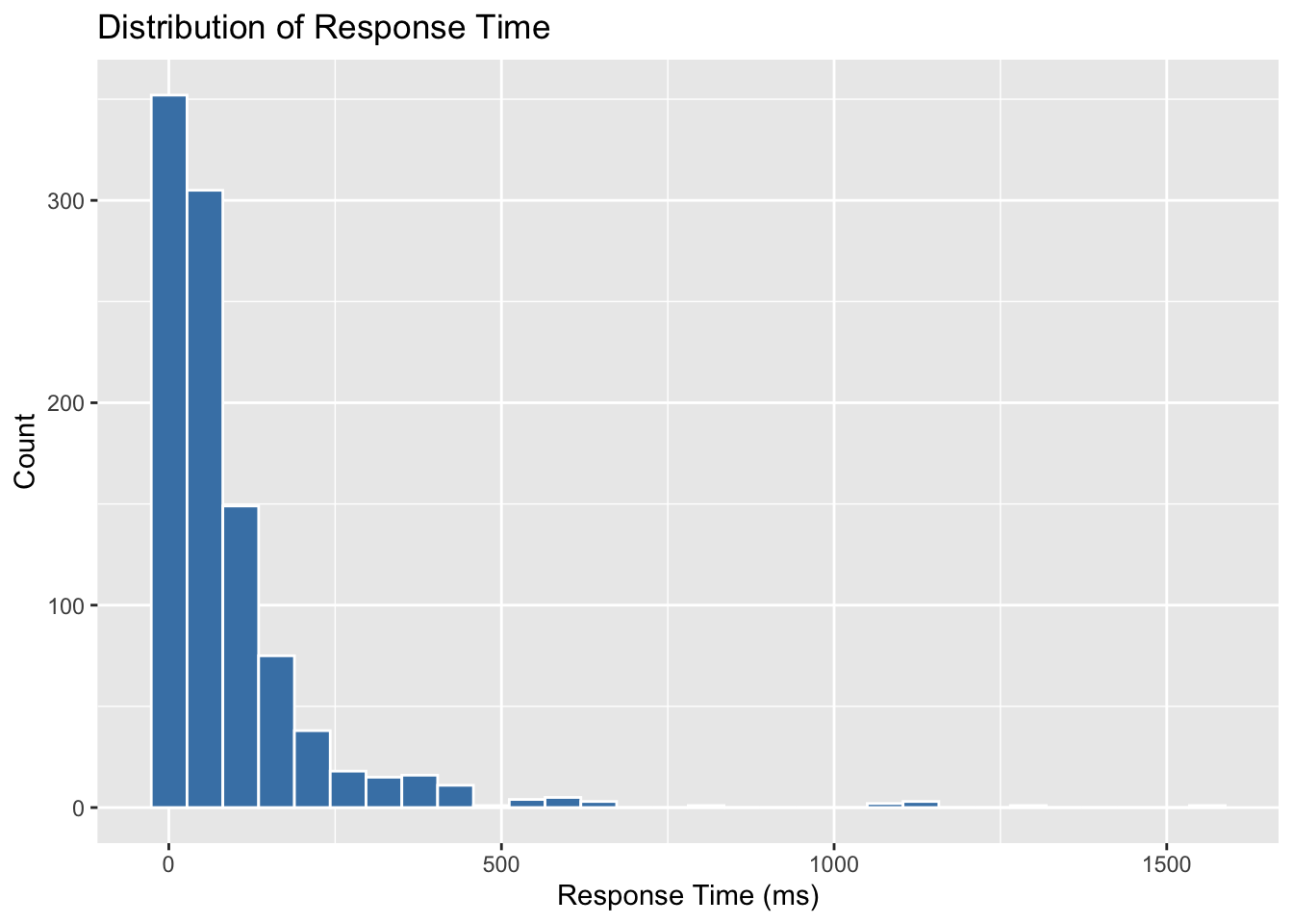
Outliers can distort regression results, so it’s always good practice to check the distribution of the response variable. In our case, we visualize response_time_ms:

R Code

library(ggplot2)

ggplot(gamma_server_encoded, aes(x = response_time_ms)) +
  geom_histogram(bins = 30, fill = "steelblue", color = "white") +
  labs(title = "Distribution of Response Time", x = "Response Time (ms)", y = "Count")

Python Code

import matplotlib.pyplot as plt
import seaborn as sns

# Histogram of response time
plt.figure(figsize=(8, 5))
sns.histplot(data_encoded["response_time_ms"], bins=30, color="steelblue", edgecolor="white")
plt.title("Distribution of Response Time")
plt.xlabel("Response Time (ms)")
plt.ylabel("Count")
plt.tight_layout()
plt.show()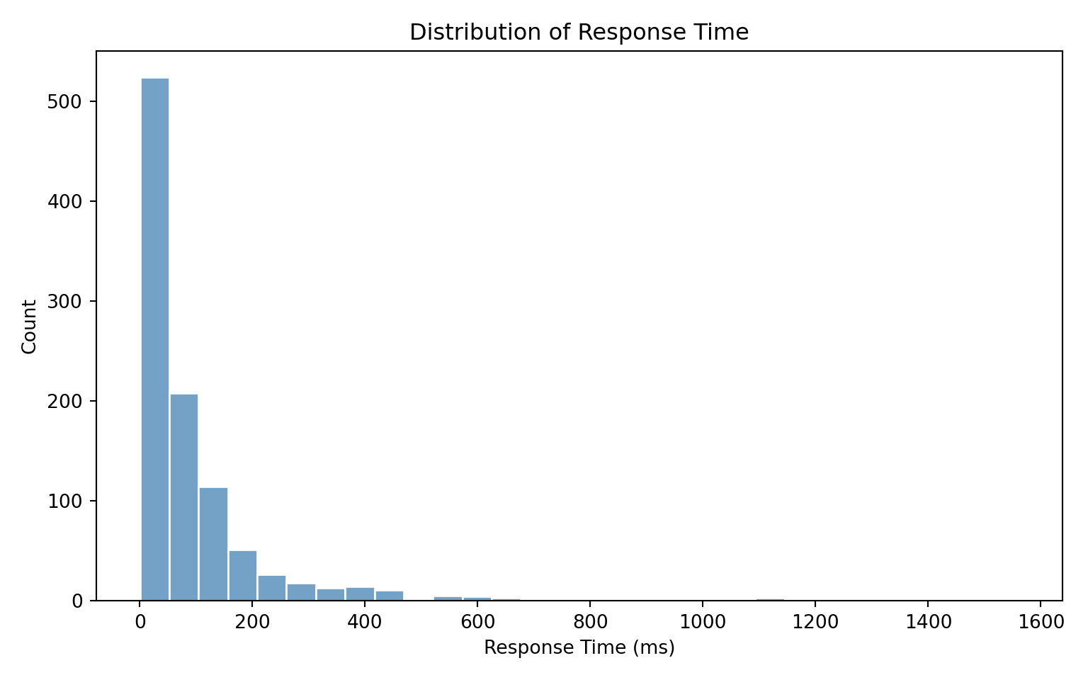

The histogram confirms that response_time_ms is right-skewed, which aligns with our expectations and supports the use of Gamma regression.

Skewed Data

It’s important to note that with Gamma-distributed data, large values in the upper tail are often part of the natural variation, not necessarily outliers to be removed. Instead of trimming them away, we rely on a model like Gamma regression that is designed to accommodate this skewness.

5. Scaling Continuous Variables (Optional)

Gamma regression does not require predictors to be on the same scale. However, scaling can sometimes help with model convergence and make coefficients easier to interpret, especially when predictors have very different ranges (for example, concurrent_users in the hundreds vs. cache_hit_rate as a percentage).

For this dataset, it may be helpful to standardize the following continuous variables:

• concurrent_users
• database_queries
• cache_hit_rate
• server_load
• memory_usage
• time_of_day

R Code

# gamma_server_encoded <- gamma_server_encoded %>%
#   mutate(across(c(concurrent_users, database_queries, cache_hit_rate, server_load, memory_usage, time_of_day), scale))

Python Code

# from sklearn.preprocessing import StandardScaler

# # List of columns to scale
# scale_cols = ["concurrent_users", "database_queries", "cache_hit_rate", "server_load", "memory_usage", "time_of_day"]

# # Initialize scaler and apply to selected columns
# scaler = StandardScaler()
# data_encoded[scale_cols] = scaler.fit_transform(data_encoded[scale_cols])

Standardizing doesn’t change the underlying fit of the Gamma regression, but it can make estimation numerically more stable and the coefficients easier to compare side by side.

After scaling, coefficients are interpreted differently: they now represent the effect of a one-standard-deviation increase in the predictor, rather than a one-unit increase.

Example of Interpretation After Scaling

Without scaling, suppose the coefficient for cache_hit_rate (measured as a percentage from 0–100) is -0.01. This means that for every 1 percentage point increase in cache hit rate, the expected response time decreases slightly.

With scaling, suppose the coefficient for cache_hit_rate becomes -0.25. This means that a one-standard-deviation increase in cache hit rate (say, about 15 percentage points in this dataset) is associated with a 0.25 decrease (on the log scale) in expected response time.

This rescaling doesn’t change the underlying relationship. It just shifts the unit of interpretation from “1 raw unit” to “1 standard deviation,” which often makes cross-variable comparisons more meaningful.

For simplicity, we will not scale the variables in this case study, but it’s a useful option to keep in mind.

A Note on Data Splitting

In many machine learning tasks, it is common to split the data into training and test sets. However, in this case study, we are not aiming to build a predictive model. Our goal is to understand how different server and request characteristics influence the average response time, which is an inferential task.

Because we are focused on interpreting the model rather than predicting new outcomes, we will use the entire dataset for model fitting. This allows us to make the best use of our data when estimating the effects of each variable.

If our goal were to build a model that predicts server response time for future requests, we would consider splitting the dataset and evaluating prediction accuracy on a holdout set.

4.9 Exploratory Data Analysis (EDA)

The data is now ready and cleaned, but before we begin modeling, it is essential to explore the dataset to understand the structure of the variables and how they relate to one another. This step, known as Exploratory Data Analysis (EDA), helps uncover patterns, identify potential issues such as skewness or outliers, and inform the modeling decisions that follow.

4.9.1 Classifying Variables

A good starting point in EDA is to classify the variables in our dataset, as this guides the choice of plots and informs how we will encode each variable when building the model.

Our response variable is:

• response_time_ms: a continuous, strictly positive variable measuring how long a server takes to respond to a request. This is well-suited for Gamma regression.

Our regressors fall into two groups:

• Continuous variables:
  • concurrent_users, database_queries, cache_hit_rate, server_load, memory_usage, time_of_day
• Categorical variables:
  • cdn_usage, request_complexity, day_of_week, geographic_region

4.9.2 Visualizing Variable Distributions

With the variables classified, we can now choose appropriate plots to explore their distributions and relationships.

Response Variable: response_time_ms

We begin by examining the distribution of the response variable.

R Code

library(ggplot2)

ggplot(gamma_server_encoded, aes(x = response_time_ms)) +
  geom_histogram(bins = 10, fill = "skyblue", color = "white") +
  labs(title = "Histogram of Response Time (ms)",
       x = "Response Time (ms)",
       y = "Frequency") +
  theme_minimal()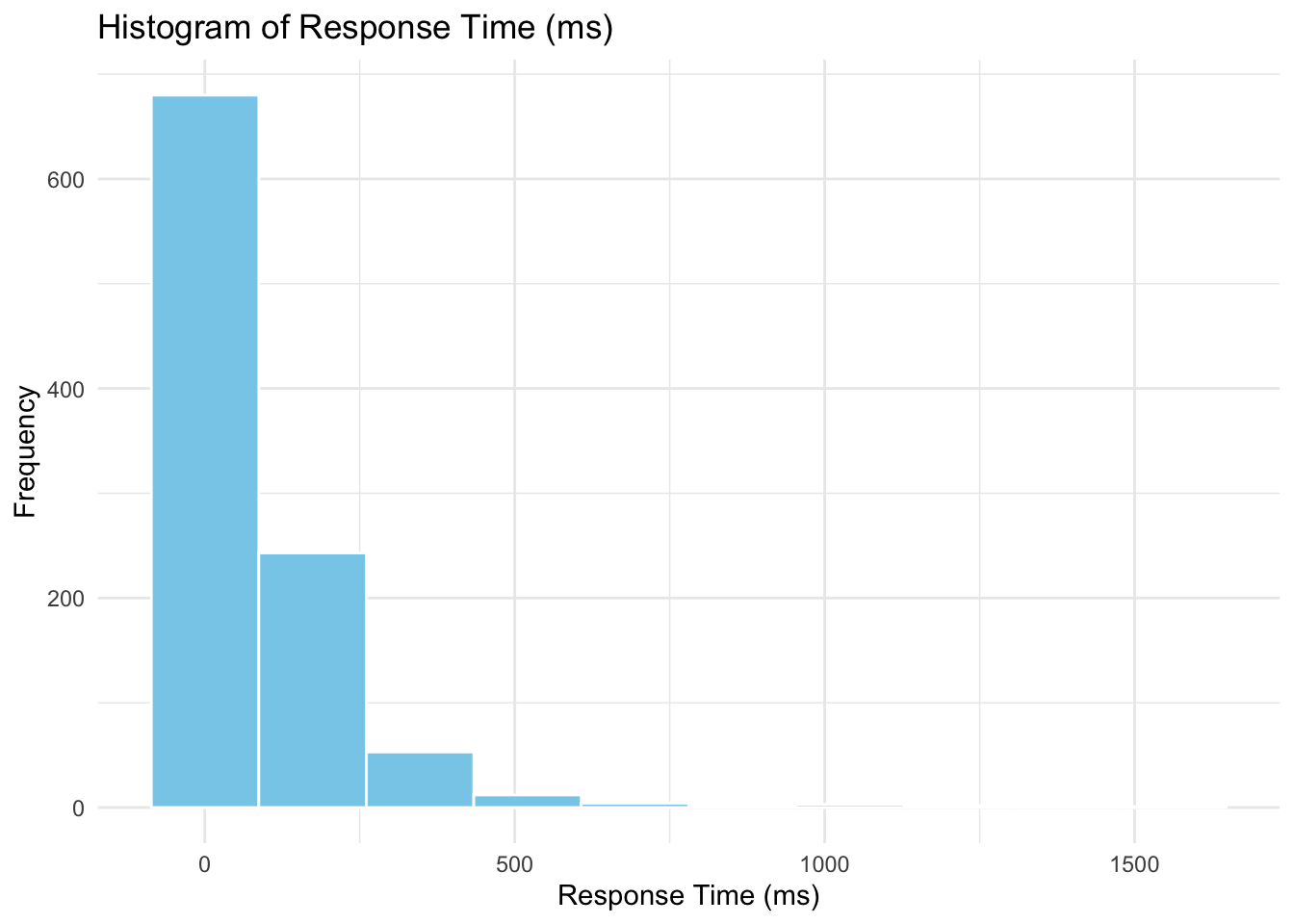

Python Code

import matplotlib.pyplot as plt
import seaborn as sns

sns.histplot(data_encoded["response_time_ms"], bins=10, kde=True, color="skyblue")
plt.title("Histogram of Response Time (ms)")
plt.xlabel("Response Time (ms)")
plt.ylabel("Frequency")
plt.tight_layout()
plt.show()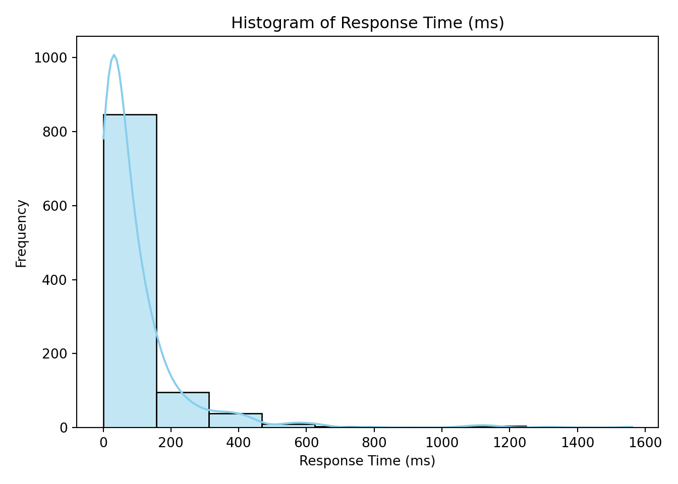

The histogram confirms that response_time_ms is strictly positive and right-skewed—just as we saw during data wrangling when we checked for negative values and visualized potential outliers.

Categorical Variables

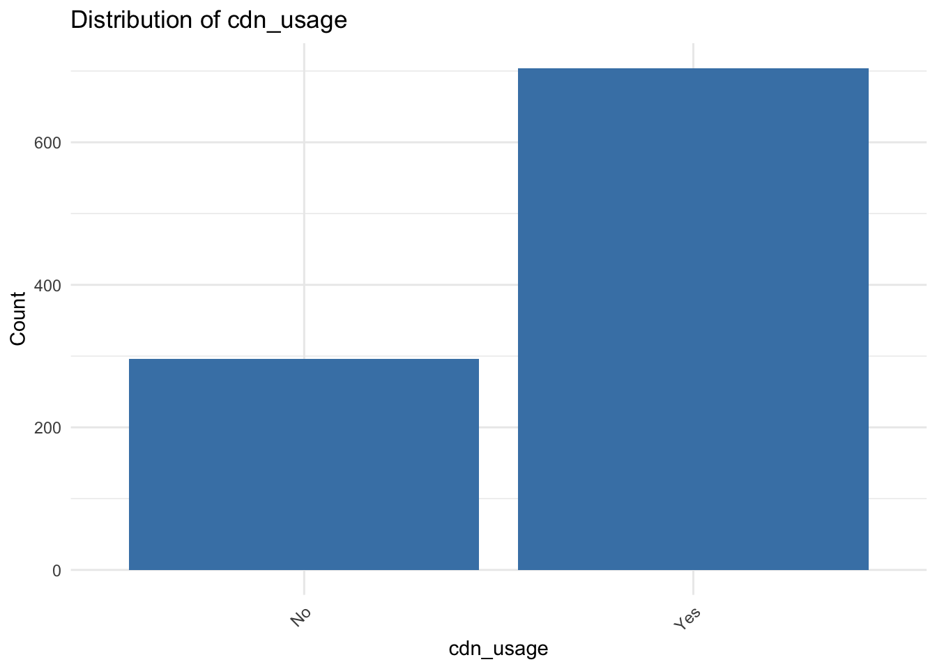
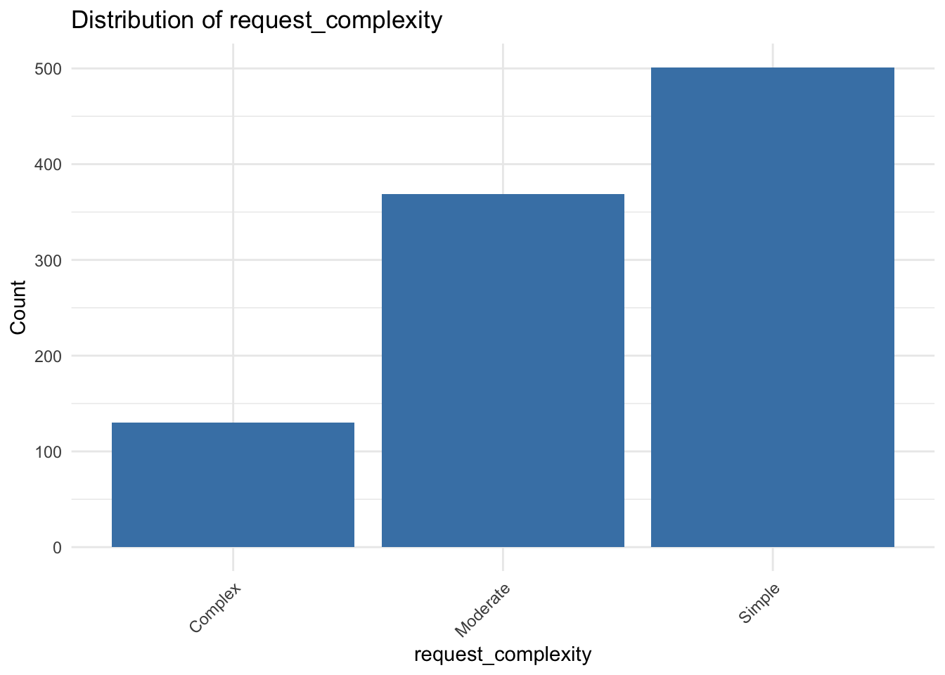
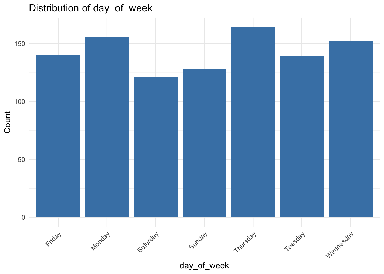
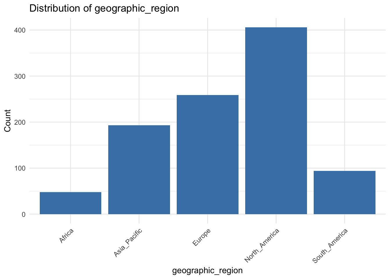
We next examine how the categorical predictors are distributed. This visualization is based on the original dataset, before encoding. Visualizing these variables helps us check if any levels are underrepresented or imbalanced, which can affect model stability and interpretation.

R Code

library(ggplot2)

categorical_vars <- c("cdn_usage", "request_complexity", "day_of_week", "geographic_region")

for (var in categorical_vars) {
  p <- ggplot(gamma_server, aes(x = .data[[var]])) +
    geom_bar(fill = "steelblue") +
    labs(
      title = paste("Distribution of", var),
      x = var,
      y = "Count"
    ) +
    theme_minimal() +
    theme(axis.text.x = element_text(angle = 45, hjust = 1))
  
  print(p)
}

Python Code

import matplotlib.pyplot as plt
import seaborn as sns

categorical_vars = ["cdn_usage", "request_complexity", "day_of_week", "geographic_region"]

for var in categorical_vars:
    sns.countplot(
        x=var,
        data=data,
        hue=var,
        palette="pastel",
        legend=False
    )
    plt.title(f"{var.replace('_', ' ').title()} Distribution")
    plt.xlabel(var.replace("_", " ").title())
    plt.ylabel("Count")
    plt.xticks(rotation=45)
    plt.tight_layout()
    plt.show()

<Axes: xlabel='cdn_usage', ylabel='count'>
Text(0.5, 1.0, 'Cdn Usage Distribution')
Text(0.5, 0, 'Cdn Usage')
Text(0, 0.5, 'Count')
([0, 1], [Text(0, 0, 'Yes'), Text(1, 0, 'No')])
<Axes: xlabel='request_complexity', ylabel='count'>
Text(0.5, 1.0, 'Request Complexity Distribution')
Text(0.5, 0, 'Request Complexity')
Text(0, 0.5, 'Count')
([0, 1, 2], [Text(0, 0, 'Moderate'), Text(1, 0, 'Complex'), Text(2, 0, 'Simple')])
<Axes: xlabel='day_of_week', ylabel='count'>
Text(0.5, 1.0, 'Day Of Week Distribution')
Text(0.5, 0, 'Day Of Week')
Text(0, 0.5, 'Count')
([0, 1, 2, 3, 4, 5, 6], [Text(0, 0, 'Saturday'), Text(1, 0, 'Thursday'), Text(2, 0, 'Monday'), Text(3, 0, 'Friday'), Text(4, 0, 'Tuesday'), Text(5, 0, 'Wednesday'), Text(6, 0, 'Sunday')])
<Axes: xlabel='geographic_region', ylabel='count'>
Text(0.5, 1.0, 'Geographic Region Distribution')
Text(0.5, 0, 'Geographic Region')
Text(0, 0.5, 'Count')
([0, 1, 2, 3, 4], [Text(0, 0, 'North_America'), Text(1, 0, 'Africa'), Text(2, 0, 'South_America'), Text(3, 0, 'Europe'), Text(4, 0, 'Asia_Pacific')])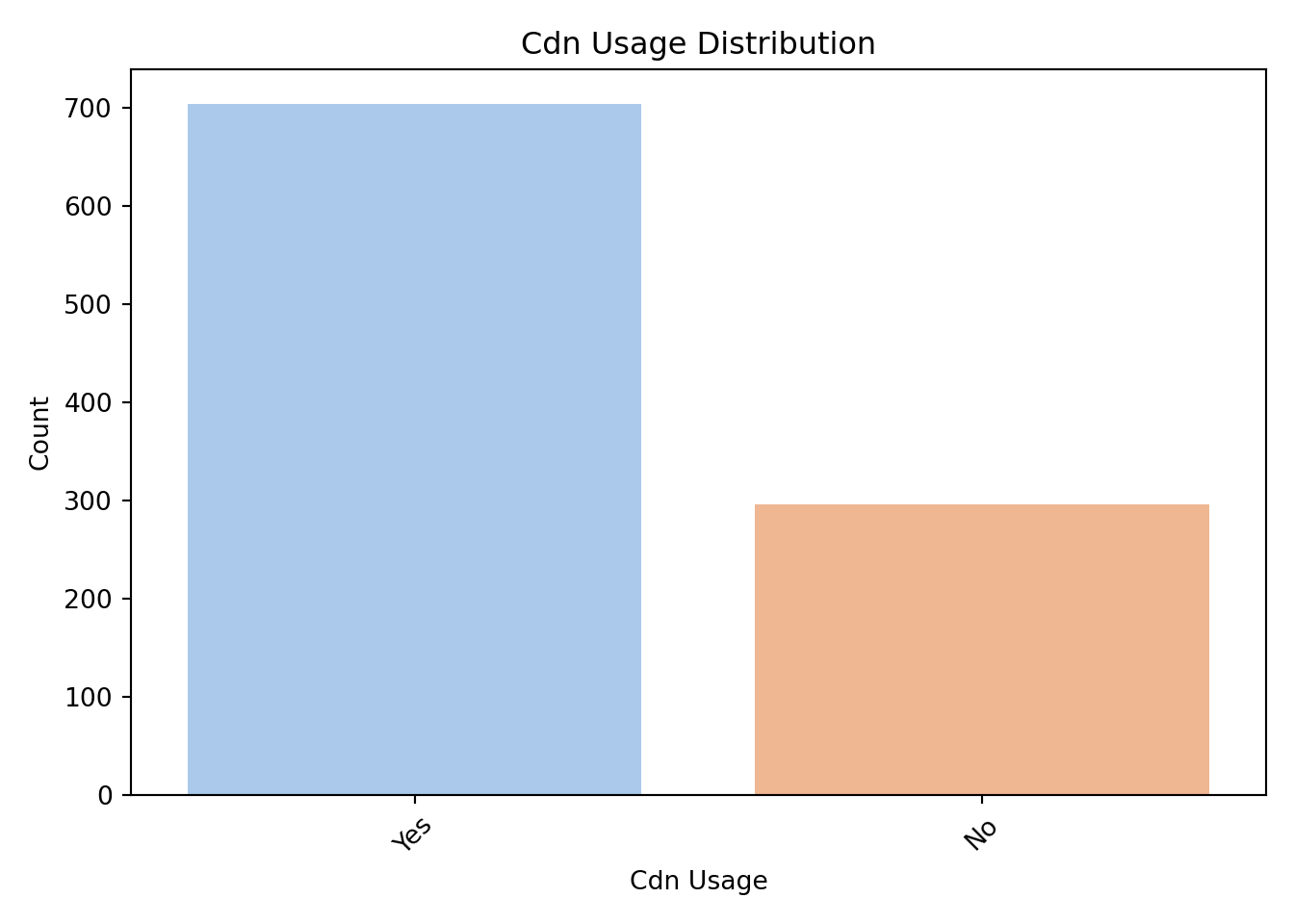

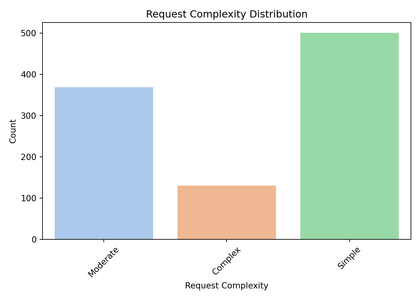
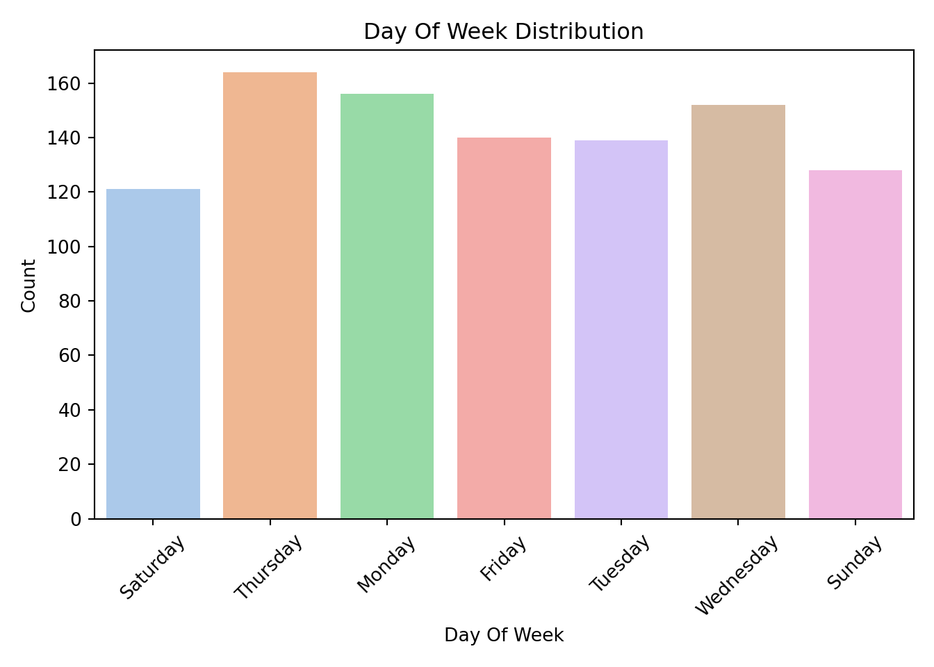
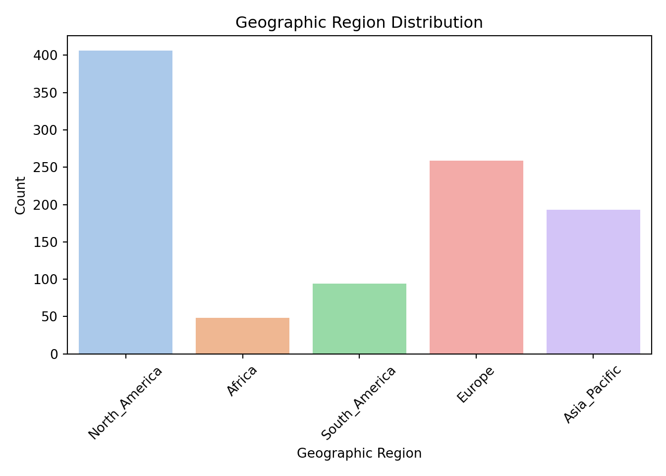
By examining these distributions, we can ensure that each category has enough observations to be meaningfully included in the model. If a category is rarely observed, it may need to be combined with others or omitted.

Numerical Variables

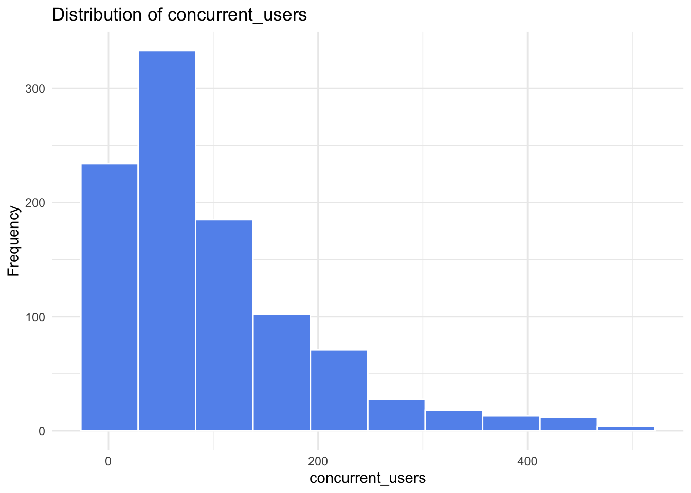
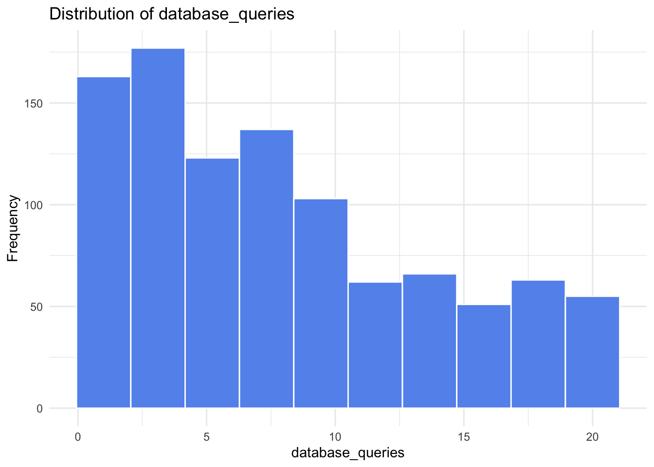
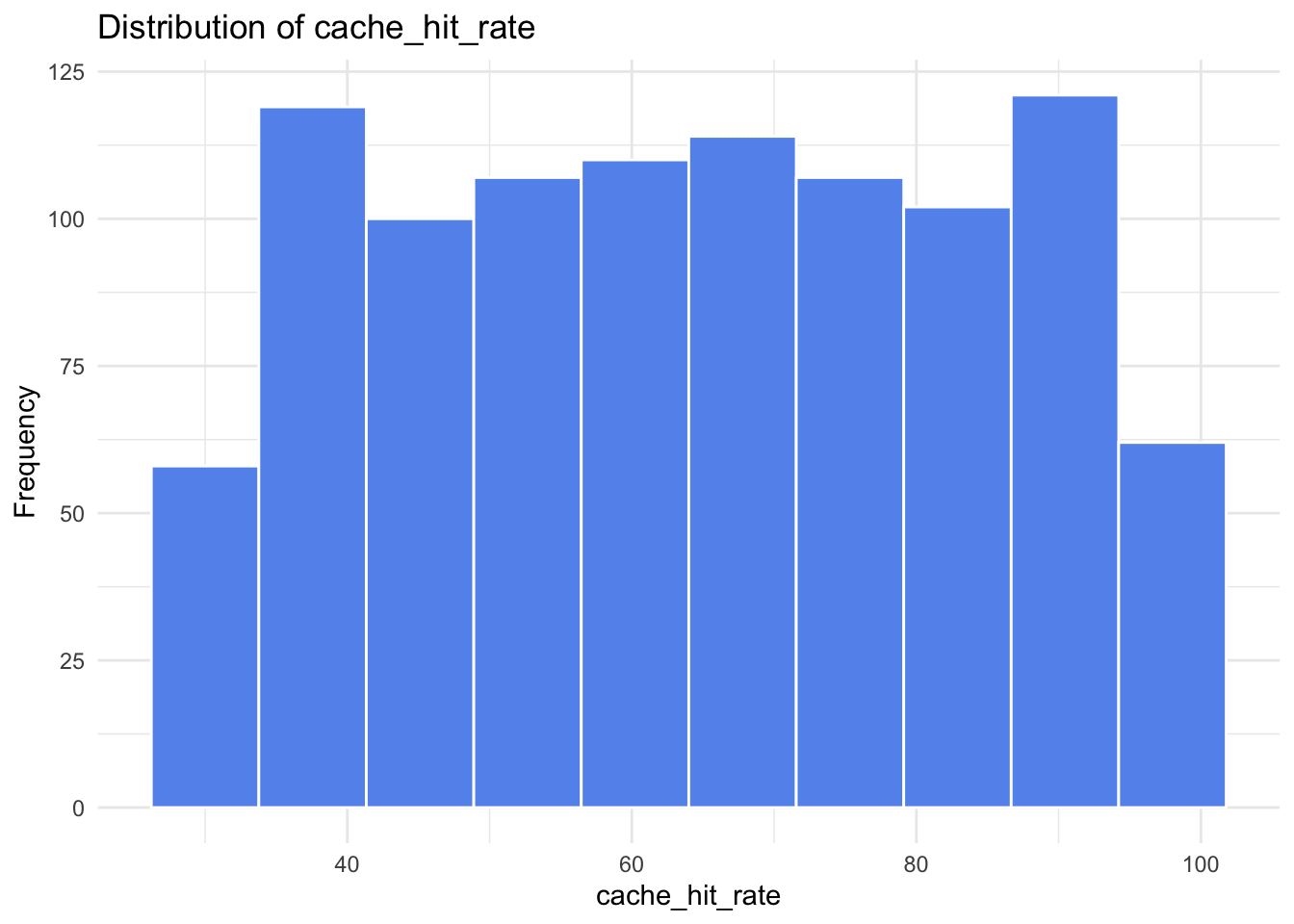
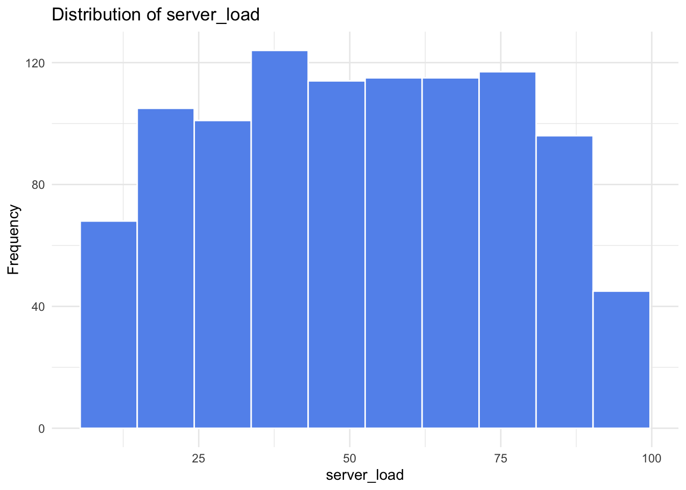
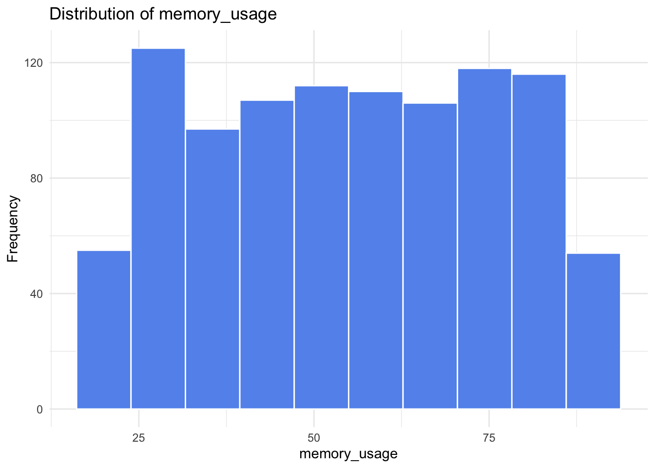
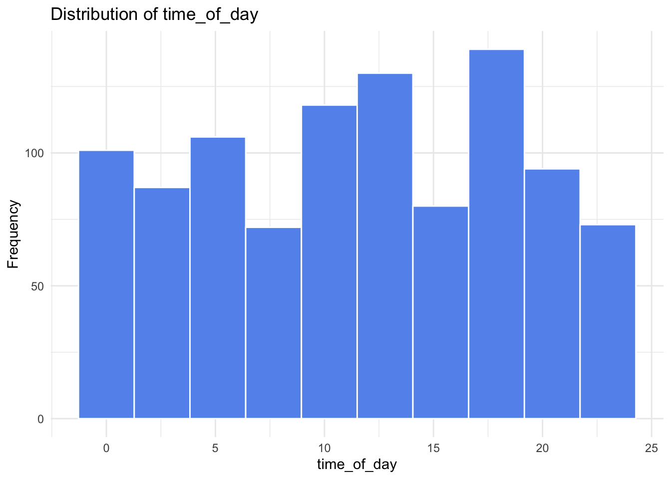
Next, we examine the distributions of the continuous predictors to understand their range, shape, and potential skewness.

R Code

library(ggplot2)

continuous_vars <- c(
  "concurrent_users", "database_queries", "cache_hit_rate",
  "server_load", "memory_usage", "time_of_day"
)

for (var in continuous_vars) {
  p <- ggplot(gamma_server, aes(x = .data[[var]])) +
    geom_histogram(bins = 10, fill = "cornflowerblue", color = "white") +
    labs(
      title = paste("Distribution of", var),
      x = var,
      y = "Frequency"
    ) +
    theme_minimal()
  
  print(p)
}

Python Code

continuous_vars = ["concurrent_users", "database_queries", "cache_hit_rate", "server_load", "memory_usage", "time_of_day"]

for var in continuous_vars:
    sns.histplot(data[var], bins=10, kde=True, color="cornflowerblue")
    plt.title(f"Distribution of {var}")
    plt.xlabel(var)
    plt.ylabel("Frequency")
    plt.tight_layout()
    plt.show()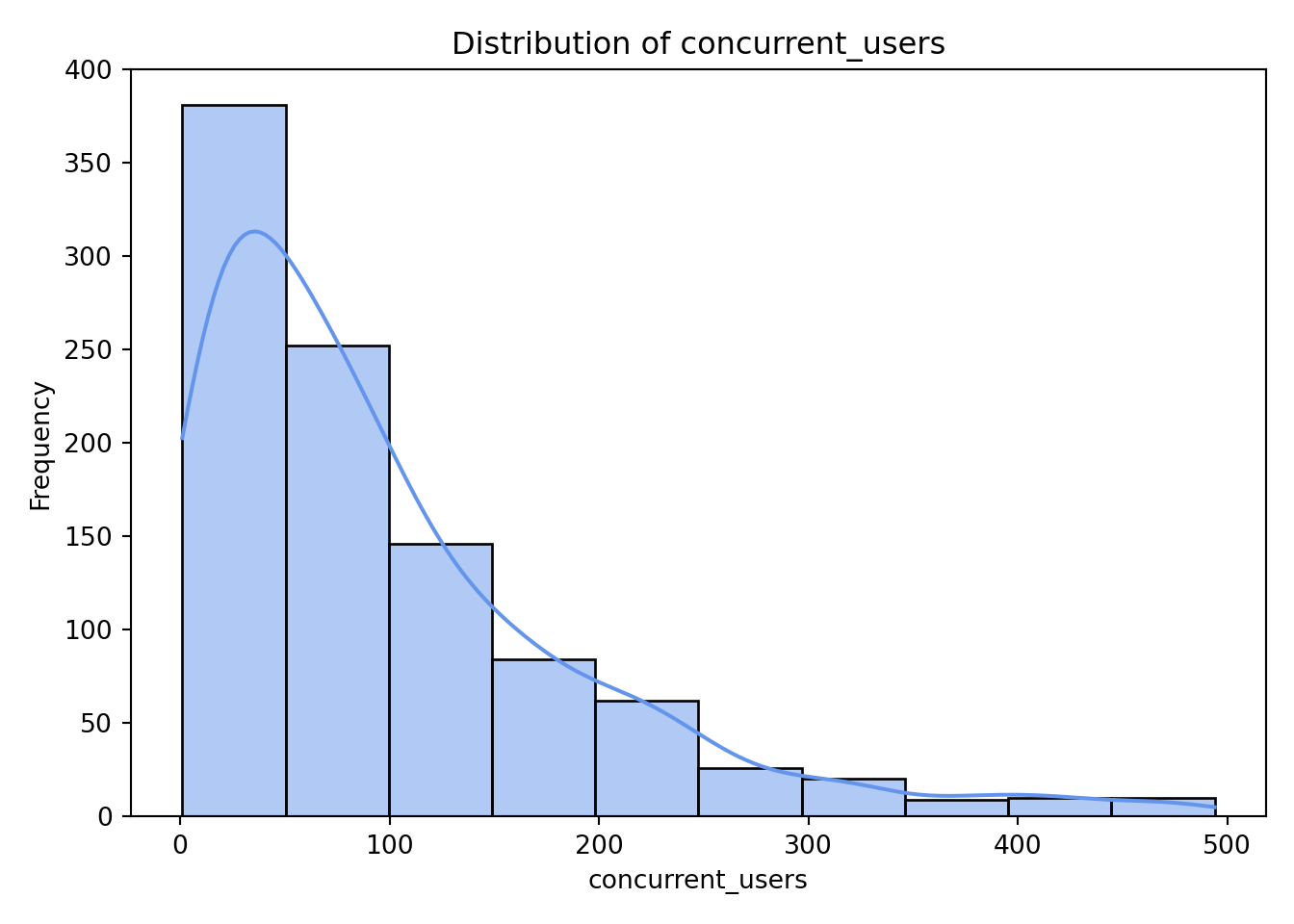

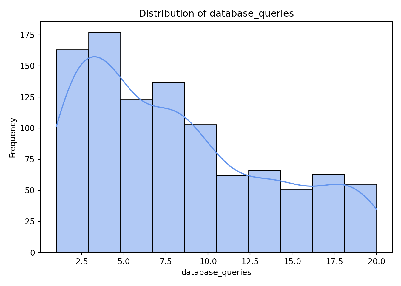
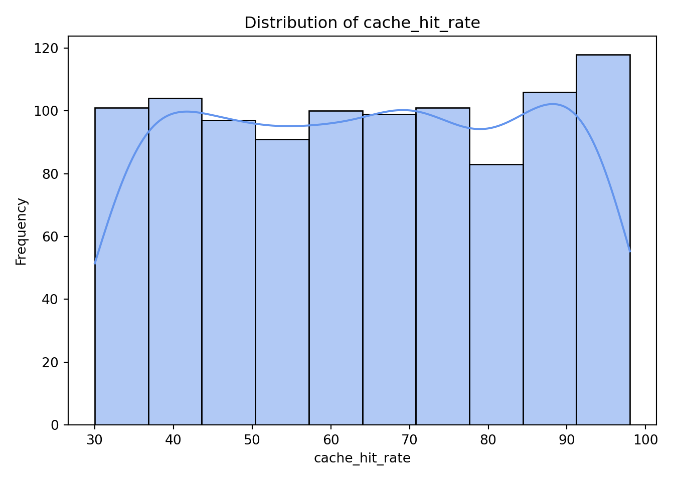
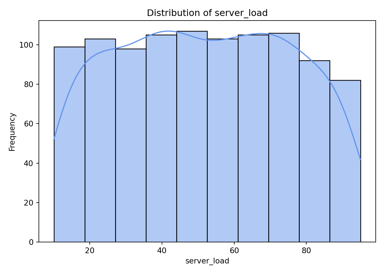
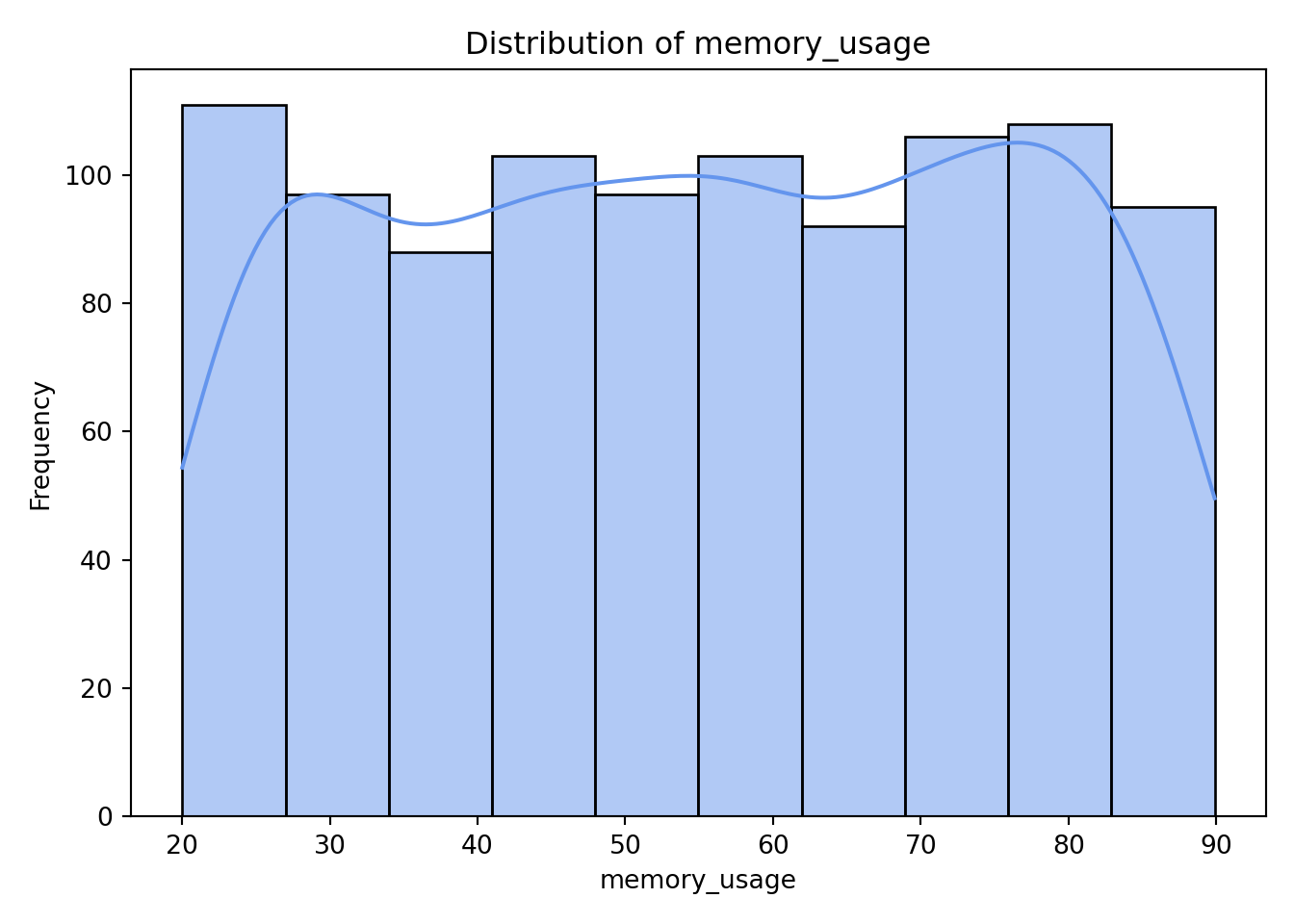
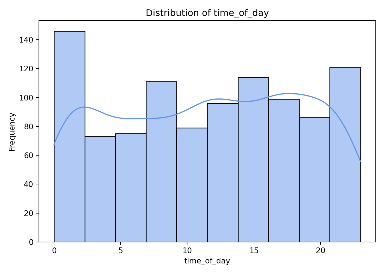
As we can see from the histograms, nothing appears too concerning. Both concurrent_users and database_queries show clear right-skewness, while the remaining continuous variables have more uniform or evenly spread distributions. memory_usage shows a lower count in its final (largest) bin, but this pattern is not unusual and does not raise any major concerns for our analysis.

4.9.3 Visualizing Predictor Relationships to Response

Having explored the univariate distributions, we can now turn to bivariate visualizations to examine how each predictor relates to the response.

Categorical Predictors vs. Response

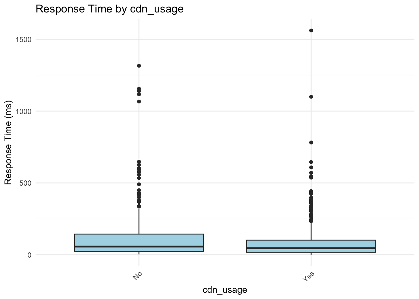
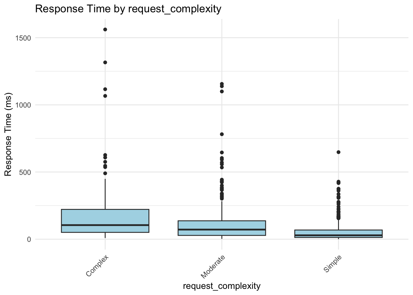
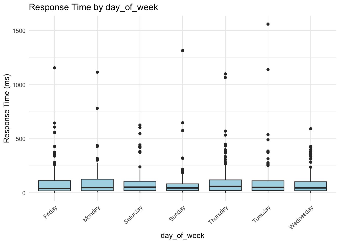
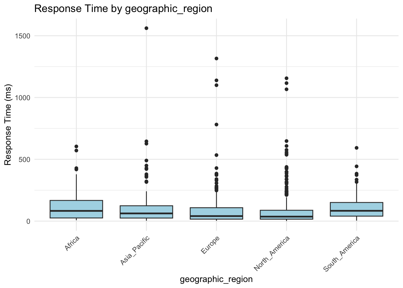
For categorical predictors, box plots provide a clear and effective way to visualize how response times vary across different groups.

R Code

categorical_vars <- c("cdn_usage", "request_complexity", "day_of_week", "geographic_region")

for (var in categorical_vars) {
  p <- ggplot(gamma_server, aes(x = .data[[var]], y = response_time_ms)) +
    geom_boxplot(fill = "lightblue") +
    labs(
      title = paste("Response Time by", var),
      x = var,
      y = "Response Time (ms)"
    ) +
    theme_minimal() +
    theme(axis.text.x = element_text(angle = 45, hjust = 1))
  
  print(p)
}

Python Code

for var in ["cdn_usage", "request_complexity", "day_of_week", "geographic_region"]:
    sns.boxplot(
        x=var,
        y="response_time_ms",
        data=data,
        hue=var,         # required if using palette
        palette="Set3",
        dodge=False      # keep single box per category
    )
    plt.legend([], [], frameon=False)  # hide duplicated legend
    plt.title(f"Response Time by {var.replace('_', ' ').title()}")
    plt.xlabel(var.replace('_', ' ').title())
    plt.ylabel("Response Time (ms)")
    plt.xticks(rotation=45)
    plt.tight_layout()
    plt.show()

<Axes: xlabel='cdn_usage', ylabel='response_time_ms'>
<matplotlib.legend.Legend object at 0x16fd58b90>
Text(0.5, 1.0, 'Response Time by Cdn Usage')
Text(0.5, 0, 'Cdn Usage')
Text(0, 0.5, 'Response Time (ms)')
([0, 1], [Text(0, 0, 'Yes'), Text(1, 0, 'No')])
<Axes: xlabel='request_complexity', ylabel='response_time_ms'>
<matplotlib.legend.Legend object at 0x16fdd0e90>
Text(0.5, 1.0, 'Response Time by Request Complexity')
Text(0.5, 0, 'Request Complexity')
Text(0, 0.5, 'Response Time (ms)')
([0, 1, 2], [Text(0, 0, 'Moderate'), Text(1, 0, 'Complex'), Text(2, 0, 'Simple')])
<Axes: xlabel='day_of_week', ylabel='response_time_ms'>
<matplotlib.legend.Legend object at 0x16ff08910>
Text(0.5, 1.0, 'Response Time by Day Of Week')
Text(0.5, 0, 'Day Of Week')
Text(0, 0.5, 'Response Time (ms)')
([0, 1, 2, 3, 4, 5, 6], [Text(0, 0, 'Saturday'), Text(1, 0, 'Thursday'), Text(2, 0, 'Monday'), Text(3, 0, 'Friday'), Text(4, 0, 'Tuesday'), Text(5, 0, 'Wednesday'), Text(6, 0, 'Sunday')])
<Axes: xlabel='geographic_region', ylabel='response_time_ms'>
<matplotlib.legend.Legend object at 0x17902a490>
Text(0.5, 1.0, 'Response Time by Geographic Region')
Text(0.5, 0, 'Geographic Region')
Text(0, 0.5, 'Response Time (ms)')
([0, 1, 2, 3, 4], [Text(0, 0, 'North_America'), Text(1, 0, 'Africa'), Text(2, 0, 'South_America'), Text(3, 0, 'Europe'), Text(4, 0, 'Asia_Pacific')])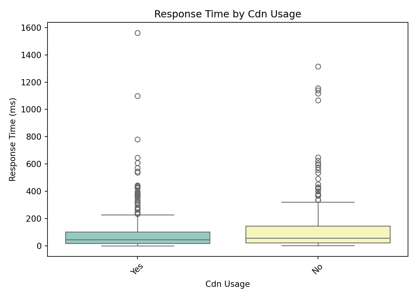

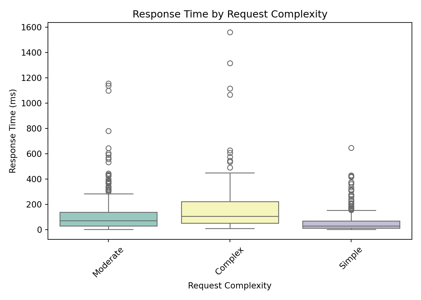
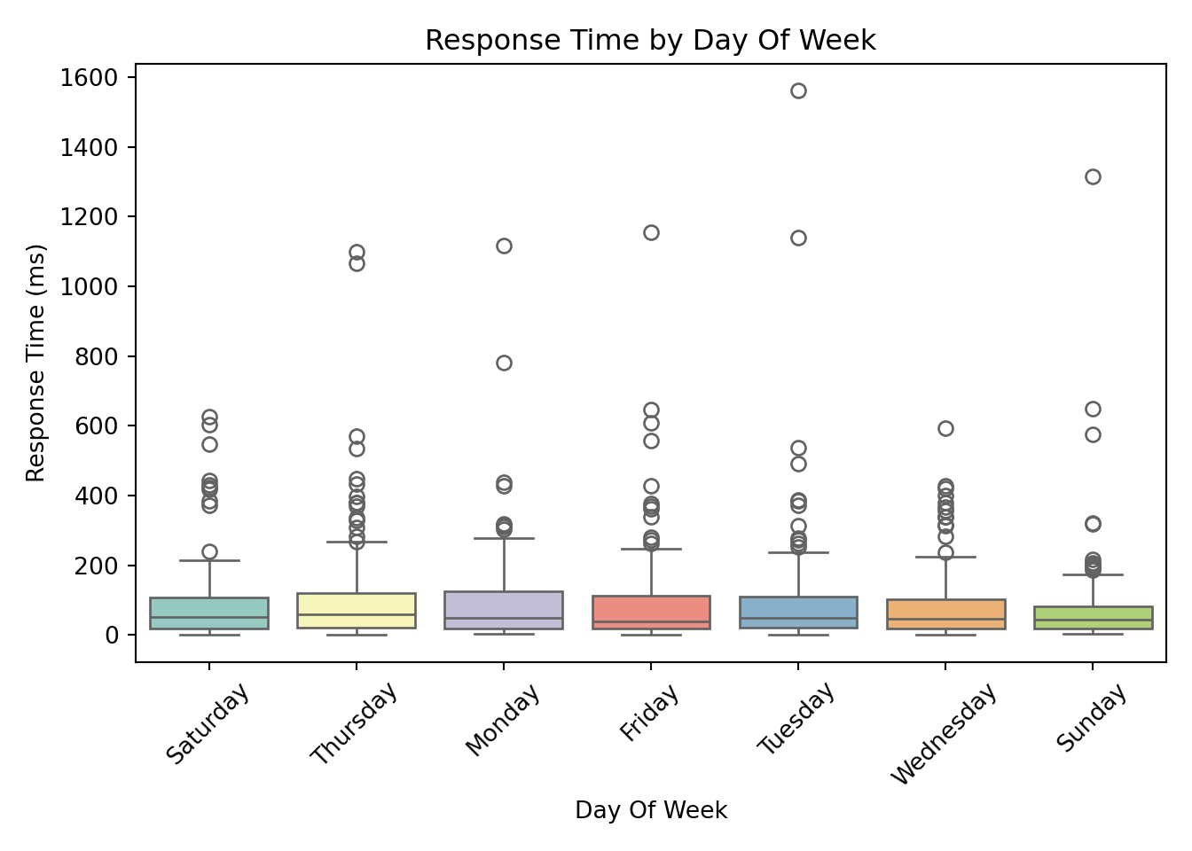
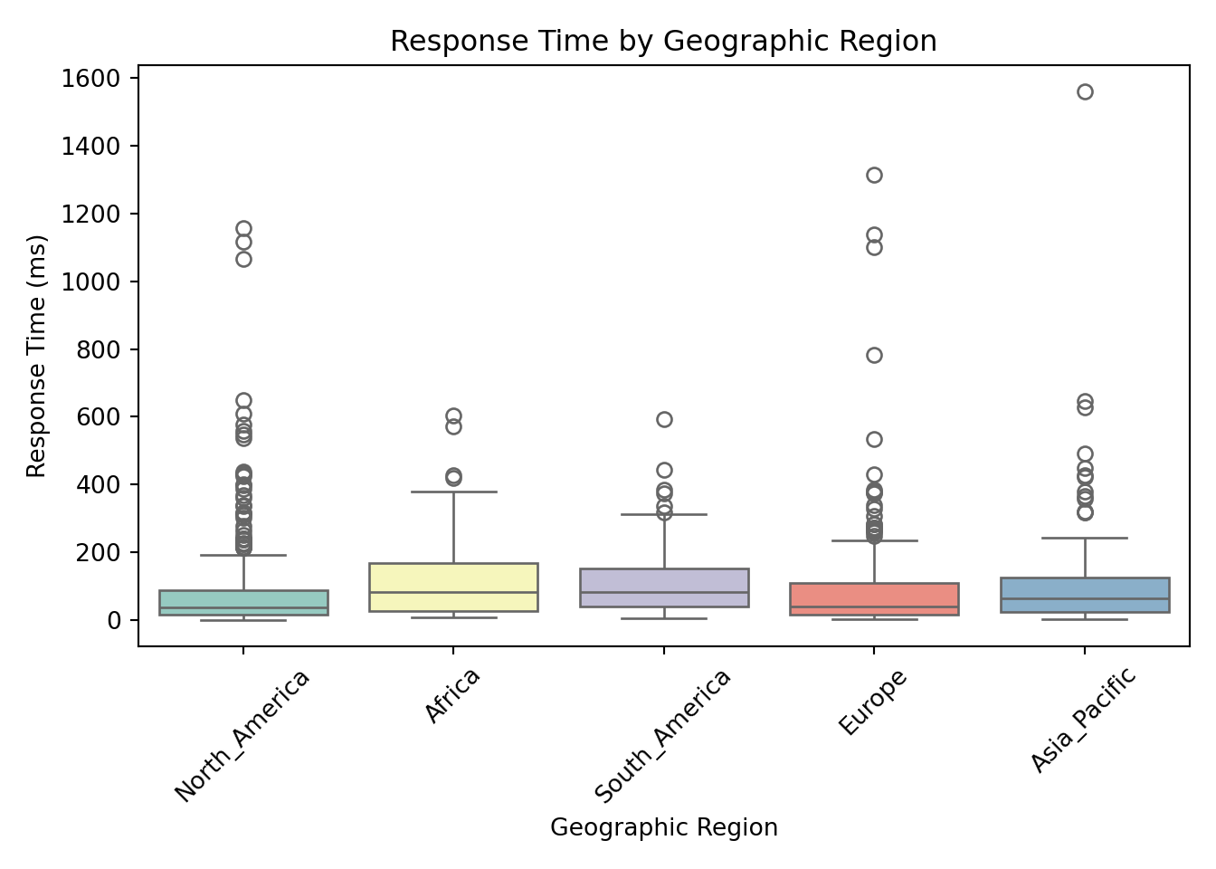
These box plots help us assess whether server response times differ meaningfully across categories. From these visualizations, request_complexity appears to have a noticeable impact on response_time_ms. At this stage, this is an educated guess based on patterns in the plots, but we’ll need statistical modeling to confirm whether the differences are truly meaningful. Apparent differences in the box plots could simply be due to random variation, limited sample size in certain groups, or interactions with other predictors.

Continuous Predictors vs. Response

For continuous predictors, scatterplots provide a clear view of how each variable is associated with the response.

R Code

continuous_vars <- c(
  "concurrent_users", "database_queries", "cache_hit_rate",
  "server_load", "memory_usage", "time_of_day"
)

for (var in continuous_vars) {
  p <- ggplot(gamma_server, aes(x = .data[[var]], y = response_time_ms)) +
    geom_point(color = "#008080") +
    geom_smooth(method = "lm", se = FALSE, color = "red") +
    labs(
      title = paste(var, "vs. Response Time"),
      x = var,
      y = "Response Time (ms)"
    ) +
    theme_minimal()
  
  print(p)
}

`geom_smooth()` using formula = 'y ~ x'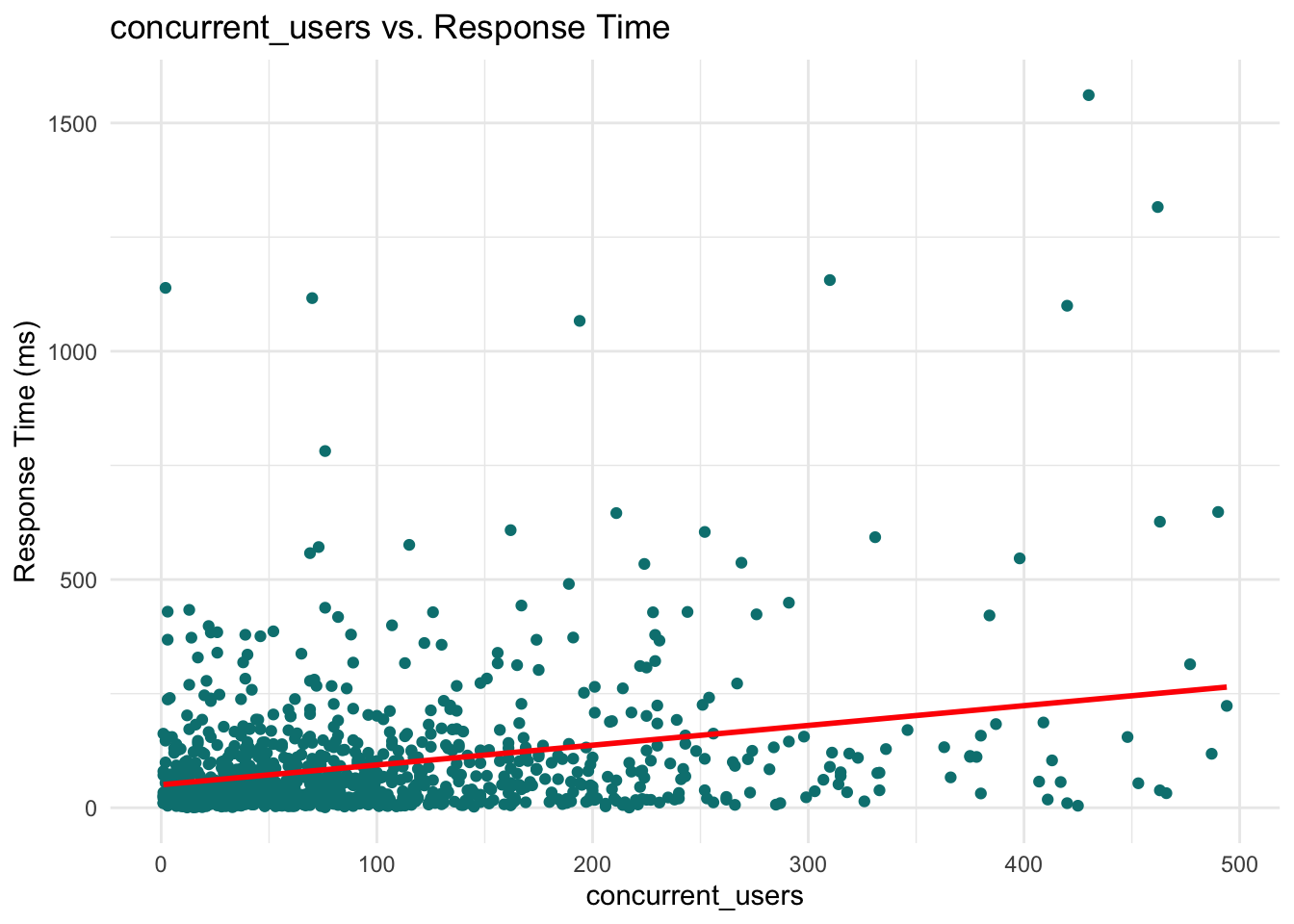

`geom_smooth()` using formula = 'y ~ x'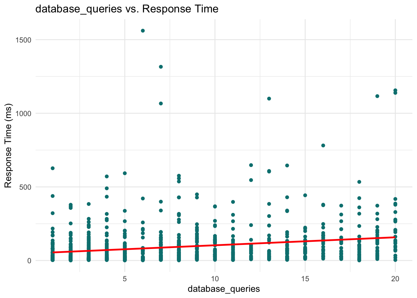

`geom_smooth()` using formula = 'y ~ x'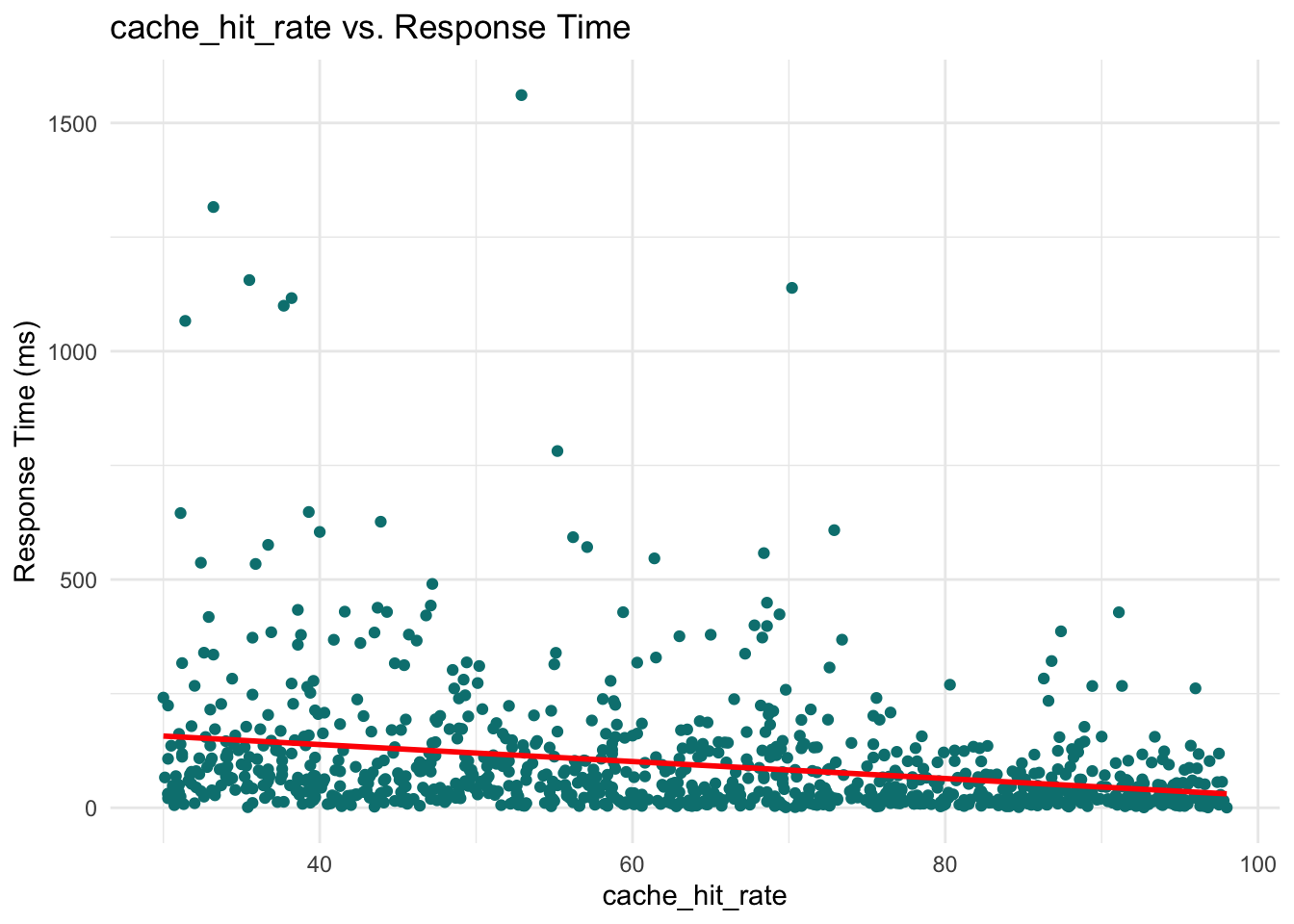

`geom_smooth()` using formula = 'y ~ x'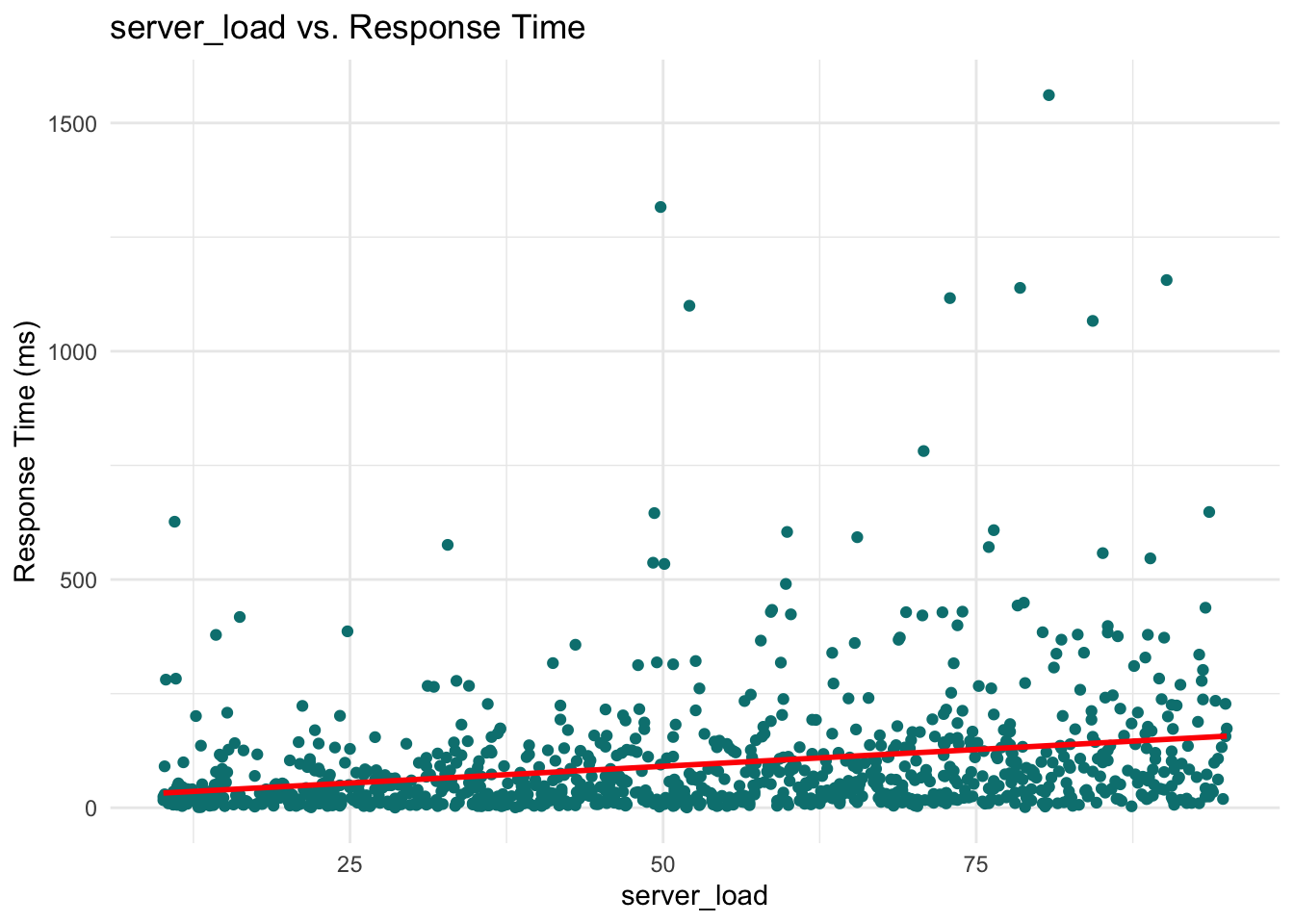

`geom_smooth()` using formula = 'y ~ x'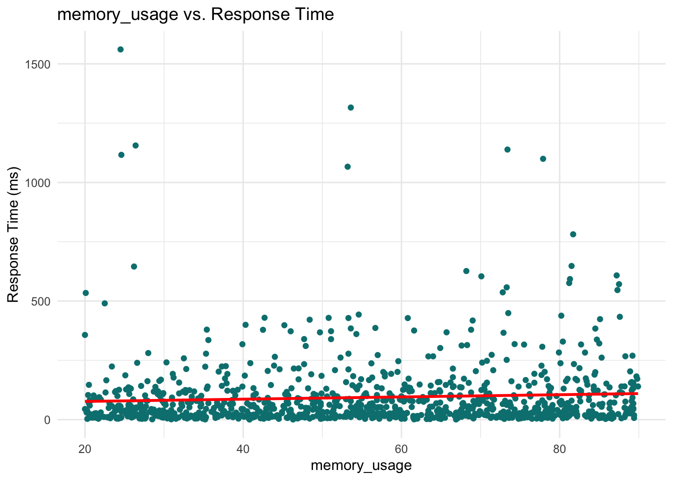

`geom_smooth()` using formula = 'y ~ x'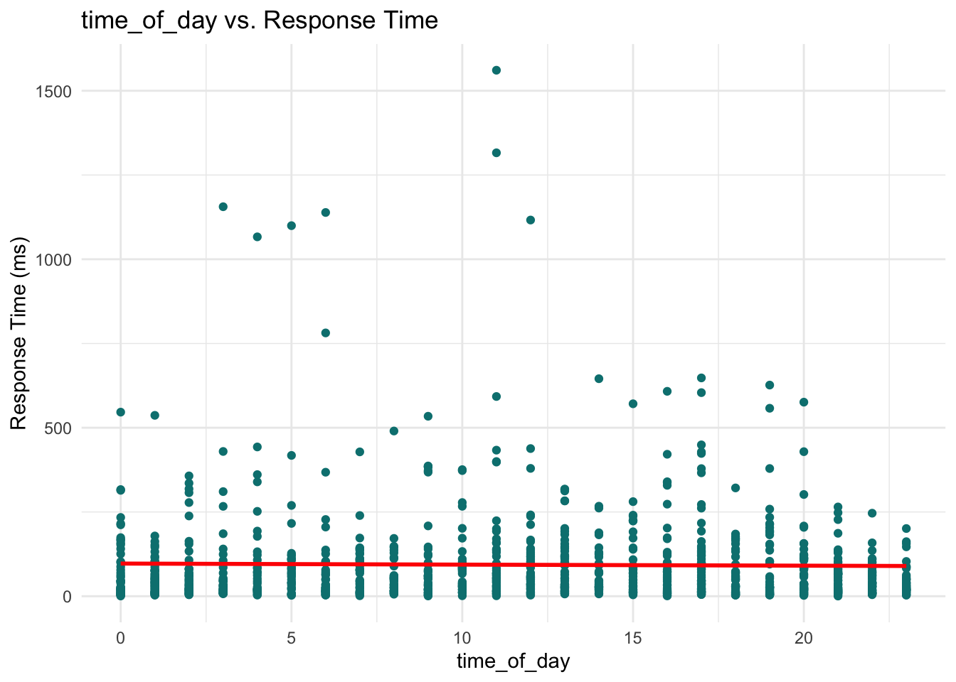

Python Code

for var in ["concurrent_users", "database_queries", "cache_hit_rate", "server_load", "memory_usage", "time_of_day"]:

    sns.scatterplot(x=var, y="response_time_ms", data=data, color="teal")
    sns.regplot(x=var, y="response_time_ms", data=data, scatter=False, color="red")
    plt.title(f"{var.replace('_', ' ').title()} vs. Response Time")
    plt.xlabel(var.replace('_', ' ').title())
    plt.ylabel("Response Time (ms)")
    plt.tight_layout()
    plt.show()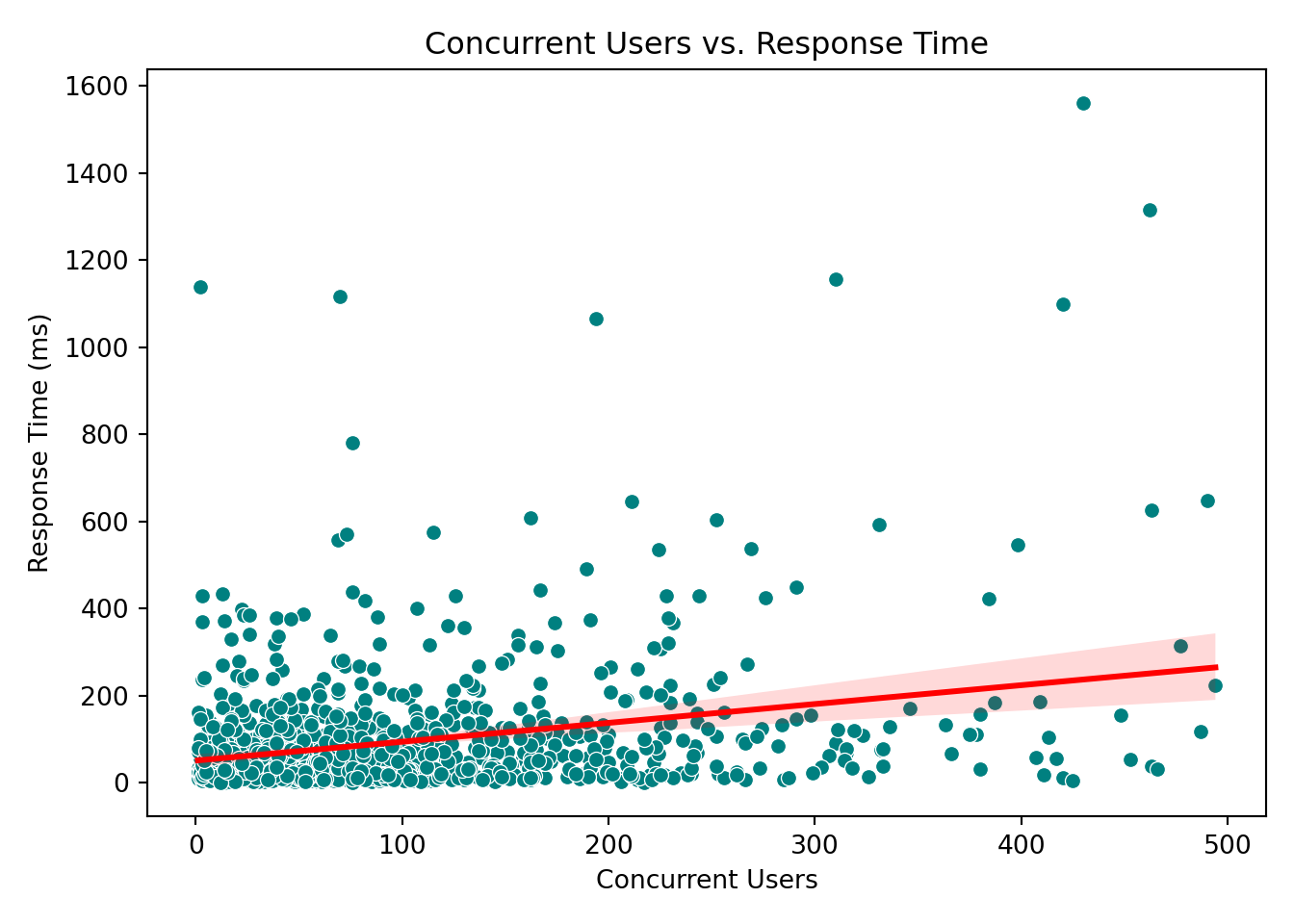

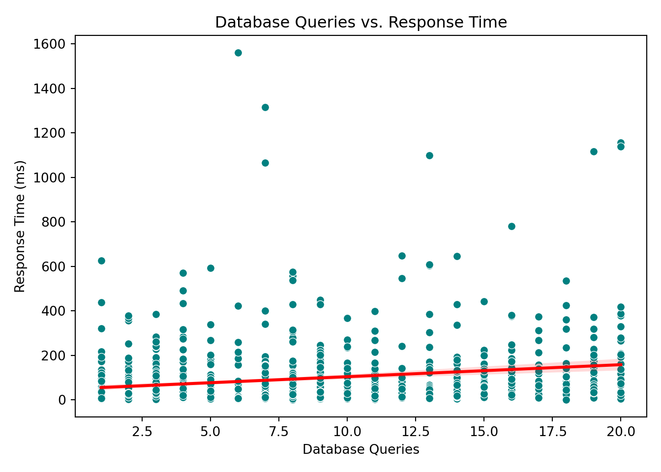
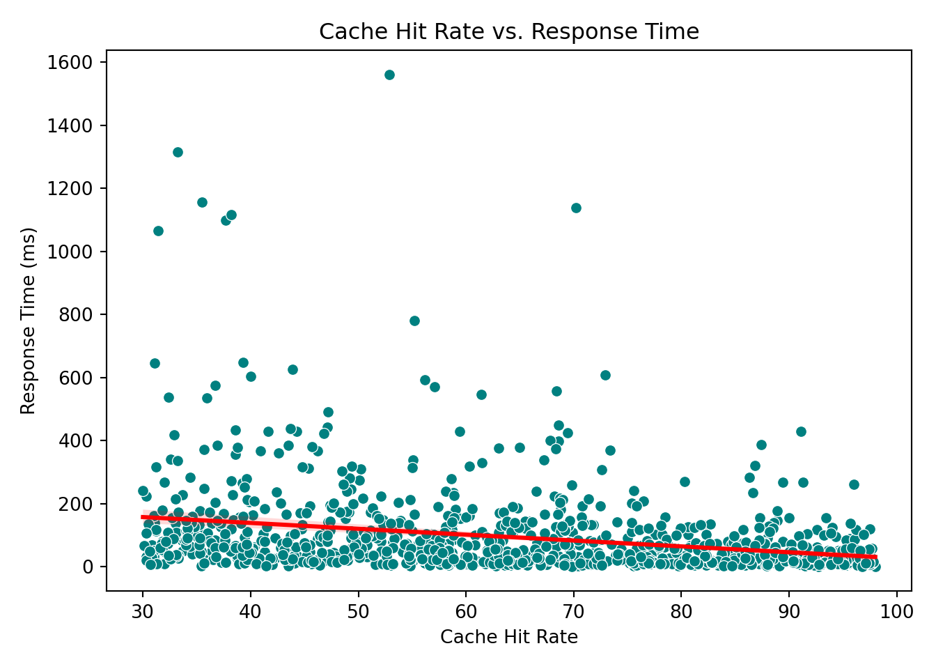
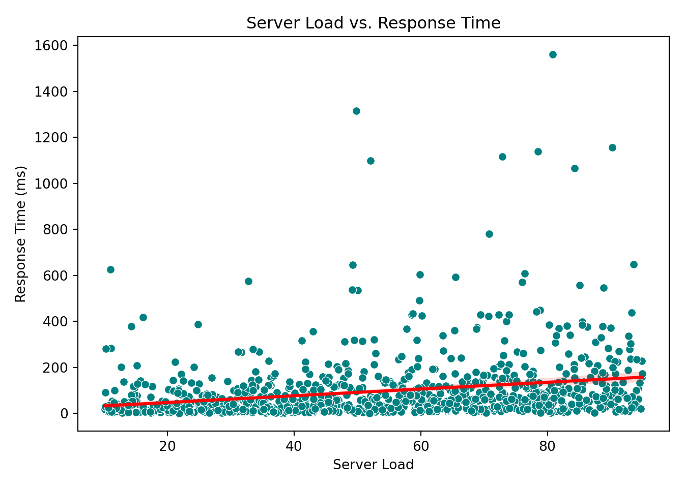
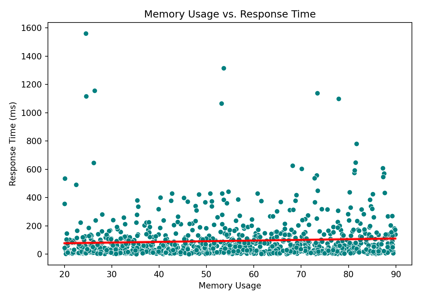
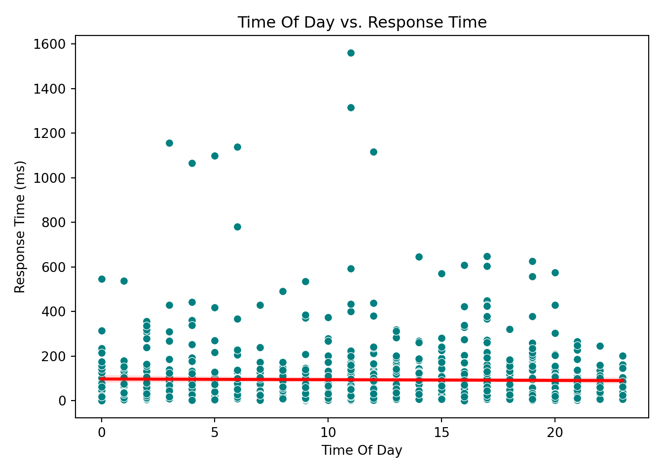
These plots help reveal trends or patterns that might inform the model structure, such as the need for transformations or interaction terms. In our case, however, none of the scatterplots show a particularly strong or obvious pattern that would suggest immediate adjustments. This is not unusual when working with skewed outcomes like response times: relationships may become clearer only after applying the link function (e.g., the log link in Gamma regression) or after controlling for multiple predictors simultaneously.

4.9.4 Key Takeaways from EDA

From our exploratory analysis, we can make a few early observations:

• The response variable (response_time_ms) is strictly positive and right-skewed, making Gamma regression an appropriate choice.
• Most requests come from North America, while Africa and South America have relatively fewer entries.
• The concurrent_users variable is also right-skewed, indicating that most requests happen under low to moderate user load, but some occur under heavy load.
• Complex requests tend to have higher response times on average, as seen in the boxplots.

These patterns help us understand the structure of the data and form preliminary hypotheses about which factors may influence response time. Keep these observations in mind. We’ll soon see whether the Gamma regression model reinforces or challenges them.

Tip

EDA is meant to explore patterns, not confirm conclusions. While these insights help guide model building, we should wait until after model fitting and diagnostics before making final interpretations.

4.10 Data Modeling

After conducting Exploratory Data Analysis (EDA), we now move into the modeling stage, where we apply a statistical model to better understand how different factors influence server response times.

4.10.1 Choosing a Suitable Regression Model

The choice of regression model depends on both the nature of the response variable and the goal of the analysis. In our case:

• The response variable, response_time_ms, is continuous, strictly positive, and right-skewed.
• The goal is to explain which factors influence the average response time, not to predict future outcomes.

Given these characteristics, a Gamma regression model with a log link is appropriate. While we had a sense of this at the beginning, the decision is best made after examining the data and understanding its distribution and structure. Once the exploratory analysis confirms positivity and skewness, Gamma regression becomes a natural choice.

Gamma regression allows us to:

• model the response in its original (positive-only) scale,
• handle right-skewed data,
• and interpret results in terms of multiplicative changes in the mean response.

In contrast, Ordinary Least Squares (OLS) assumes constant variance and symmetry around the mean, assumptions that clearly do not hold in this dataset. This makes Gamma regression a more suitable and robust option for our analysis.

4.10.2 Defining Modeling Parameters

With the model selected, our next step is to specify the variables that will go into the equation. In this analysis, we use all available predictors. Together, these variables capture a mix of technical metrics (e.g., server load, memory usage), behavioral context (e.g., request complexity, time of day), and infrastructure details (e.g., CDN usage, geographic region). Using the full set of variables provides a well-rounded view of the factors that may influence response time. Therefore, we will include all predictors in the model.

4.10.3 Setting Up the Modeling Equation

By including all predictors in the Gamma regression, we arrive at the following model equation. This equation represents the log of the average response time as a linear function of the predictors.

\[ \begin{align*} \log(\mu_i) &= \beta_0 \\ &\quad + \beta_1 \times \text{concurrent\_users}_i \\ &\quad + \beta_2 \times \text{database\_queries}_i \\ &\quad + \beta_3 \times \text{cache\_hit\_rate}_i \\ &\quad + \beta_4 \times \text{server\_load}_i \\ &\quad + \beta_5 \times \text{memory\_usage}_i \\ &\quad + \beta_6 \times \text{time\_of\_day}_i \\ &\quad + \beta_7 \times \text{cdn\_usage}_i \\ &\quad + \beta_8 \times \text{request\_complexity}_i \\ &\quad + \beta_9 \times \text{day\_of\_week}_i \\ &\quad + \beta_{10} \times \text{geographic\_region}_i \end{align*} \]

The beauty of mathematics is that we can then back-transform the predicted value from the log scale using the exponential function:

\[ \mu_i = \exp(\text{linear combination of predictors}) \]

where:

• \(\mu_i\) is the expected average response time for the \(i\)-th request
  
• \(\beta_0\) is the intercept
  
• \(\beta_1, \beta_2, \ldots \beta_{10}\) are the coefficients for each predictor

This means that each coefficient (\(\beta_n\)) describes the multiplicative effect on the mean response time:

• \(\beta_1\): How response time changes as the number of concurrent users increases
  
• \(\beta_7\): The impact of CDN usage versus not using a CDN
  
• \(\beta_8\): How request complexity levels (Moderate or Simple) compare to the base level (Complex)
  
• \(\beta_{10}\): Regional differences in server response behavior

This model structure allows us to capture both technical and contextual effects on server performance using a regression framework suited for positive and skewed outcomes.

4.11 Estimation

With the data modeling stage completed, we now move on to estimation, where we actually fit the Gamma regression model to the data and obtain numerical estimates for each coefficient. These estimates allow us to quantify how each predictor influences the average server response time under the specified model.

How Gamma Regression Is Fit

Unlike OLS, which minimizes squared errors, Gamma regression relies on maximum likelihood estimation (MLE). MLE is more appropriate when the outcome is strictly positive and right-skewed, as it takes into account the distributional assumptions of the Gamma model.

4.11.1 Fitting the Model

In R, you can use the glm() function with family = Gamma(link = "log"). In Python, we use statsmodels with the Gamma family and log link:

R Code

# Load required library
library(stats)

# Fit Gamma regression model
gamma_model <- glm(
  response_time_ms ~ concurrent_users + database_queries + cache_hit_rate +
    server_load + time_of_day + memory_usage +
    day_of_week_Monday + day_of_week_Saturday + day_of_week_Sunday +
    day_of_week_Thursday + day_of_week_Tuesday + day_of_week_Wednesday +
    geographic_region_Asia_Pacific + geographic_region_Europe +
    geographic_region_North_America + geographic_region_South_America +
    request_complexity_Moderate + request_complexity_Simple +
    cdn_usage_Yes,
  family = Gamma(link = "log"),
  data = gamma_server_encoded
)

# Display model summary
summary(gamma_model)

Call:
glm(formula = response_time_ms ~ concurrent_users + database_queries + 
    cache_hit_rate + server_load + time_of_day + memory_usage + 
    day_of_week_Monday + day_of_week_Saturday + day_of_week_Sunday + 
    day_of_week_Thursday + day_of_week_Tuesday + day_of_week_Wednesday + 
    geographic_region_Asia_Pacific + geographic_region_Europe + 
    geographic_region_North_America + geographic_region_South_America + 
    request_complexity_Moderate + request_complexity_Simple + 
    cdn_usage_Yes, family = Gamma(link = "log"), data = gamma_server_encoded)

Coefficients:
                                  Estimate Std. Error t value Pr(>|t|)    
(Intercept)                      4.7603924  0.1971945  24.141  < 2e-16 ***
concurrent_users                 0.0029522  0.0002651  11.134  < 2e-16 ***
database_queries                 0.0737204  0.0045095  16.348  < 2e-16 ***
cache_hit_rate                  -0.0192125  0.0012367 -15.536  < 2e-16 ***
server_load                      0.0171491  0.0010331  16.599  < 2e-16 ***
time_of_day                      0.0020302  0.0035487   0.572  0.56740    
memory_usage                     0.0096178  0.0012127   7.931 5.91e-15 ***
day_of_week_Monday              -0.0353228  0.0908594  -0.389  0.69754    
day_of_week_Saturday            -0.1781832  0.0968001  -1.841  0.06596 .  
day_of_week_Sunday              -0.2334680  0.0954806  -2.445  0.01465 *  
day_of_week_Thursday            -0.1025488  0.0899490  -1.140  0.25453    
day_of_week_Tuesday              0.0298651  0.0932648   0.320  0.74887    
day_of_week_Wednesday           -0.0845206  0.0909808  -0.929  0.35312    
geographic_region_Asia_Pacific  -0.3520001  0.1261621  -2.790  0.00537 ** 
geographic_region_Europe        -0.5514433  0.1226661  -4.495 7.77e-06 ***
geographic_region_North_America -0.7498536  0.1193010  -6.285 4.91e-10 ***
geographic_region_South_America -0.1160509  0.1385021  -0.838  0.40229    
request_complexity_Moderate     -0.5889707  0.0797133  -7.389 3.17e-13 ***
request_complexity_Simple       -1.3210568  0.0768739 -17.185  < 2e-16 ***
cdn_usage_Yes                   -0.3824307  0.0542098  -7.055 3.27e-12 ***
---
Signif. codes:  0 '***' 0.001 '**' 0.01 '*' 0.05 '.' 0.1 ' ' 1

(Dispersion parameter for Gamma family taken to be 0.6007392)

    Null deviance: 1447.44  on 999  degrees of freedom
Residual deviance:  565.82  on 980  degrees of freedom
AIC: 10028

Number of Fisher Scoring iterations: 6

Python Code

import statsmodels.api as sm
import statsmodels.formula.api as smf

# Fit Gamma regression model using log link
gamma_model = smf.glm(
    formula="""
        response_time_ms ~ concurrent_users + database_queries + cache_hit_rate +
        server_load + time_of_day + memory_usage +
        day_of_week_Monday + day_of_week_Saturday + day_of_week_Sunday +
        day_of_week_Thursday + day_of_week_Tuesday + day_of_week_Wednesday +
        geographic_region_Asia_Pacific + geographic_region_Europe +
        geographic_region_North_America + geographic_region_South_America +
        request_complexity_Moderate + request_complexity_Simple +
        cdn_usage_Yes
    """,
    data=data_encoded,
    family=sm.families.Gamma(link=sm.families.links.log())
).fit()

/Users/alexi/Library/Caches/org.R-project.R/R/reticulate/uv/cache/archive-v0/QyZZds9PnwYenrsdCGRmj/lib/python3.11/site-packages/statsmodels/genmod/families/links.py:13: FutureWarning: The log link alias is deprecated. Use Log instead. The log link alias will be removed after the 0.15.0 release.
  warnings.warn(

# Display model summary
print(gamma_model.summary())

                 Generalized Linear Model Regression Results                  
==============================================================================
Dep. Variable:       response_time_ms   No. Observations:                 1000
Model:                            GLM   Df Residuals:                      980
Model Family:                   Gamma   Df Model:                           19
Link Function:                    log   Scale:                         0.60074
Method:                          IRLS   Log-Likelihood:                -4996.9
Date:                Sat, 15 Aug 2026   Deviance:                       565.82
Time:                        00:50:33   Pearson chi2:                     589.
No. Iterations:                    17   Pseudo R-squ. (CS):             0.7695
Covariance Type:            nonrobust                                         
===========================================================================================================
                                              coef    std err          z      P>|z|      [0.025      0.975]
-----------------------------------------------------------------------------------------------------------
Intercept                                   4.7604      0.197     24.140      0.000       4.374       5.147
day_of_week_Monday[T.True]                 -0.0353      0.091     -0.389      0.697      -0.213       0.143
day_of_week_Saturday[T.True]               -0.1782      0.097     -1.841      0.066      -0.368       0.012
day_of_week_Sunday[T.True]                 -0.2335      0.095     -2.445      0.014      -0.421      -0.046
day_of_week_Thursday[T.True]               -0.1026      0.090     -1.140      0.254      -0.279       0.074
day_of_week_Tuesday[T.True]                 0.0299      0.093      0.320      0.749      -0.153       0.213
day_of_week_Wednesday[T.True]              -0.0845      0.091     -0.929      0.353      -0.263       0.094
geographic_region_Asia_Pacific[T.True]     -0.3520      0.126     -2.790      0.005      -0.599      -0.105
geographic_region_Europe[T.True]           -0.5514      0.123     -4.495      0.000      -0.792      -0.311
geographic_region_North_America[T.True]    -0.7499      0.119     -6.285      0.000      -0.984      -0.516
geographic_region_South_America[T.True]    -0.1161      0.139     -0.838      0.402      -0.388       0.155
request_complexity_Moderate[T.True]        -0.5890      0.080     -7.389      0.000      -0.745      -0.433
request_complexity_Simple[T.True]          -1.3211      0.077    -17.185      0.000      -1.472      -1.170
cdn_usage_Yes[T.True]                      -0.3824      0.054     -7.055      0.000      -0.489      -0.276
concurrent_users                            0.0030      0.000     11.134      0.000       0.002       0.003
database_queries                            0.0737      0.005     16.348      0.000       0.065       0.083
cache_hit_rate                             -0.0192      0.001    -15.536      0.000      -0.022      -0.017
server_load                                 0.0171      0.001     16.599      0.000       0.015       0.019
time_of_day                                 0.0020      0.004      0.572      0.567      -0.005       0.009
memory_usage                                0.0096      0.001      7.931      0.000       0.007       0.012
===========================================================================================================

4.11.2 Interpreting the Coefficients

The modelling was a success! Based on our estimates, the fitted equation is as follow:

\[ \begin{align*} \log(\mu) &= 5.85 \\ &\quad + 0.276 \times \text{concurrent\_users} \\ &\quad + 0.407 \times \text{database\_queries} \\ &\quad - 0.384 \times \text{cache\_hit\_rate} \\ &\quad + 0.411 \times \text{server\_load} \\ &\quad + 0.197 \times \text{memory\_usage} \\ &\quad + \cdots \\ &\quad - 0.116 \times \text{geographic\_region\_South\_America} \end{align*} \]

4.12 Goodness of Fit

All of the numbers above look encouraging, but it’s important to make sure they are reliable. Before drawing conclusions, we need to check whether the model has successfully captured the main patterns in the data, or whether it’s missing something important. This brings us to the next stage: goodness of fit, where we evaluate how well the Gamma regression model represents the underlying data.

4.12.1 Deviance Residuals vs. Fitted Values

In generalized linear models like Gamma regression, we use something called deviance residuals to examine goodness of fit. These are special residuals that account for the type of model we’re using. They’re designed to help us detect if the model is systematically making mistakes.

Definition of Deviance Residual

Deviance Residuals measure how far each observation is from what the model expects, using the correct distribution (in this case, the Gamma distribution). You can think of it as:

A standardized measure of “how surprising” each data point is under the fitted model.

Some key points:

• Deviance residuals are always centered around zero.
• Large positive or negative values indicate observations the model struggles to fit.
• Patterns in a residual–fitted plot can reveal model misspecification (e.g., wrong link function, missing predictors, nonlinear relationships).

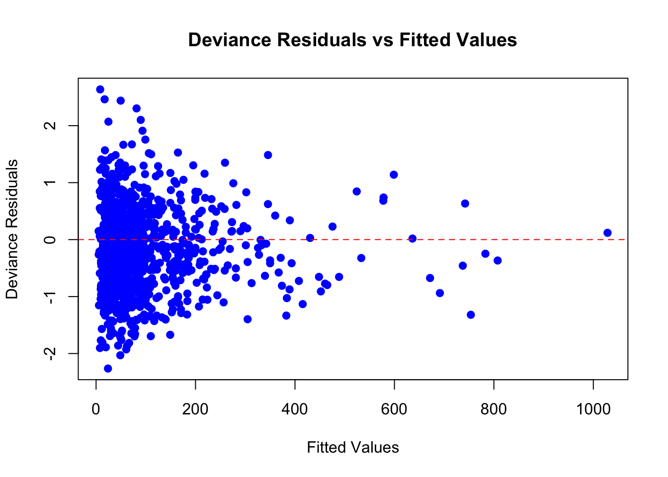
Below is a plot of deviance residuals against the model’s fitted values (the predicted average response time for each observation):

R Code

# Plot deviance residuals vs fitted values
plot(gamma_model$fitted.values, residuals(gamma_model, type = "deviance"),
     main = "Deviance Residuals vs Fitted Values",
     xlab = "Fitted Values",
     ylab = "Deviance Residuals",
     pch = 19, col = "blue")
abline(h = 0, lty = 2, col = "red")

Python Code

import matplotlib.pyplot as plt
import statsmodels.api as sm

# Fitted values and deviance residuals
fitted_values = gamma_model.fittedvalues
deviance_residuals = gamma_model.resid_deviance

# Plot
plt.scatter(fitted_values, deviance_residuals, color="blue", s=30)
plt.axhline(0, linestyle="--", color="red")
plt.title("Deviance Residuals vs Fitted Values")
plt.xlabel("Fitted Values")
plt.ylabel("Deviance Residuals")
plt.tight_layout()
plt.show()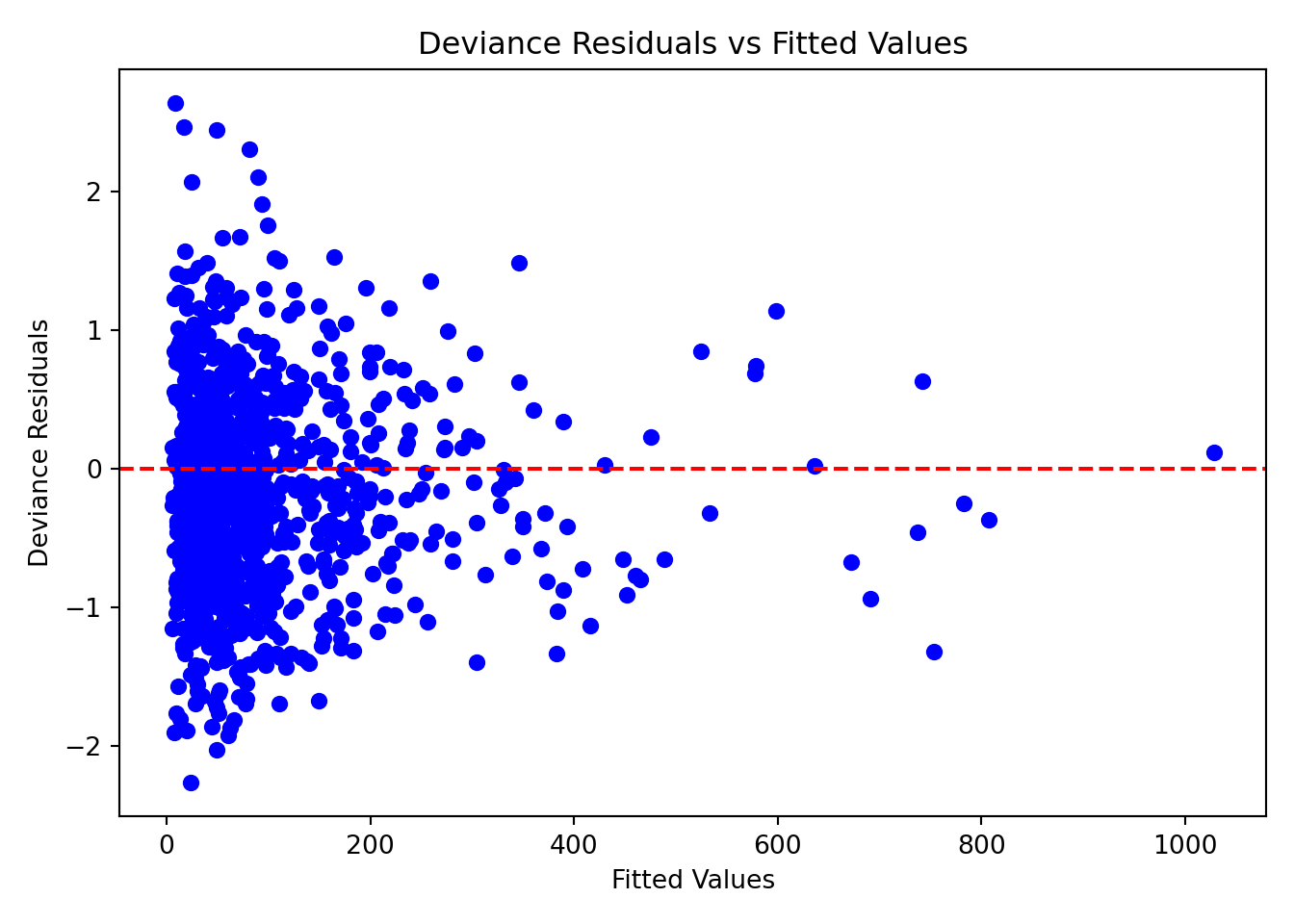

In a well-fitting model, we expect the deviance residuals to be centered around zero, without any noticeable patterns or trends, and to be spread out fairly evenly across the range of fitted values. When we look at this plot, it meets these expectations quite well.

Why the Spread Looks Flat

You might expect residuals to spread out more as the predicted value increases, especially in a Gamma model, where variance increases with the mean. But remember: deviance residuals have already been scaled to account for that.

That’s why the spread of points looks more even instead of fanning outward. This is actually a good sign. It tells us the model is appropriately handling the increasing variability.

4.12.2 Deviance and AIC

The deviance residual plot helps us see whether individual observations behave as the model expects. However, residuals only tell part of the story. They show where the model fits well or poorly, but not how well the model fits overall.

To assess overall model quality, we turn to model-level deviance, which summarizes the total remaining error after fitting the Gamma regression.

Residual Deviance

In linear regression, we often use the sum of squared errors to summarize model fit. In Gamma regression, an analogous measure is deviance, which quantifies the discrepancy between the model and the observed data in a way appropriate for the Gamma distribution.

There are two key deviance values:

• Null deviance is the error from a model that uses only the overall mean response time.
• Residual deviance is the error remaining after fitting the Gamma regression with all predictors included.

We also compare this to the null deviance, which is the error you’d get if the model only used the overall average and ignored all predictors.

Here are the values from our analysis:

• Null deviance: 1447.44
  
• Residual deviance: 565.82

The large drop from the null deviance to the residual deviance indicates that our predictors substantially improve the model’s ability to explain variation in response time.

AIC (Akaike Information Criterion)

Another useful summary statistic is the Akaike Information Criterion (AIC). You can think of AIC as a score that balances two goals:

• How well the model fits the data
  
• How simple the model is (fewer predictors = simpler)

A lower AIC indicates a better overall balance between fit and complexity. Our model’s AIC is:

• AIC: 10028

This number isn’t very informative on its own. It becomes meaningful when we compare it to the AIC of alternative models (for example, a model with fewer predictors or a different link function). In such comparisons, the model with the lower AIC is preferred, because it captures the data more efficiently without unnecessary complexity.

4.13 Results

With the goodness-of-fit checks completed, we can be reasonably confident that our model provides a reliable representation of the data. Now we can return to our original question:

What factors influence the average response time of a server?

Before interpreting the coefficients, remember that we used a Gamma regression with a log link. This means that, unlike ordinary least squares, coefficients operate multiplicatively on the original scale: a one-unit change in a predictor corresponds to a percentage change in the expected response time, holding all other variables constant.

4.13.1 Statistically Significant Predictors

Several predictors in our model have p-values less than 0.05, which means there is strong statistical evidence that they influence average server response time:

• Concurrent users: The coefficient is 0.276. This means for each additional concurrent user, the expected response time increases by a factor of \(e^{0.276} \approx 1.32\), or 32%. This is a substantial increase.

• Database queries: With a coefficient of 0.407, each additional database query increases the response time by a factor of \(e^{0.407} \approx 1.50\), or 50%. More queries mean heavier processing load.

• Cache hit rate: The coefficient is \(-0.384\). This means that a one-unit increase in cache hit rate (e.g., from 60% to 61%) is associated with a decrease in response time by \(e^{-0.384} \approx 0.68\), or 32%.

• Server load: The coefficient is 0.411. This corresponds to a 50.9% increase in response time per unit increase in server load (\(e^{0.411} \approx 1.51\)), which aligns with intuition.

• Memory usage: This has a positive coefficient of 0.197. Each unit increase in memory usage increases expected response time by \(e^{0.197} \approx 1.22\), or 22%.

• CDN usage: The coefficient is \(-0.382\). Using a content delivery network is associated with a 31.8% decrease in expected response time (\(e^{-0.382} \approx 0.68\)).

• Request complexity (Moderate and Simple): Compared to complex requests, moderate requests reduce response time by about 44.7% (\(e^{-0.589} \approx 0.55\)), and simple requests reduce it by about 73.4% (\(e^{-1.321} \approx 0.27\)).

• Geographic region: Requests from Asia Pacific, Europe, and North America all show significantly shorter response times compared to the reference region. For example, the coefficient for North America is \(-0.750\), meaning a 52.8% shorter response time on average (\(e^{-0.750} \approx 0.47\)).

4.13.2 Non-Significant Predictors

The following predictors have p-values greater than 0.05 and are not statistically significant in this model:

• Time of day: This does not appear to have a measurable effect on response time.

• Day of week: Most weekday indicators are not significant, suggesting that response time is consistent across the week.

• South America: The coefficient is small and the p-value is high, indicating no strong evidence of different response times compared to the baseline region.

These variables might still play a role in different datasets or under different modeling assumptions, but here they do not provide strong enough evidence to conclude an effect.

Interpretation Reminder

These effects represent associations, not causal guarantees. They reflect average differences after adjusting for other predictors in the model. System-level performance is complex, and real-world behavior may involve interactions or nonlinearities not captured here.

4.14 Storytelling

Finally, to wrap up the workflow, the final step is to consider how the results can actually be used. This part of the workflow is often referred to as storytelling, where we connect the analysis back to practical decision-making.

The Gamma regression model highlights several factors that consistently influence server response times. Packaging these findings into insights helps different stakeholders like engineers, product teams, and managers make informed decisions. Below, we translate the model’s results into practical implications.

4.14.1 Key Insights From the Model

System load emerges as one of the strongest drivers of slower performance. Variables such as concurrent users, database queries, and server load all increase response time substantially, especially under peak conditions. These results suggest that heavy user traffic and complex queries consistently create processing bottlenecks. To mitigate these issues, teams should invest in more robust load balancing, optimize query performance, and refine autoscaling strategies to better accommodate traffic spikes.

Caching proves to be one of the most powerful levers for improving response times. Both cache hit rate and CDN usage lead to substantial reductions in latency, indicating that even small improvements in caching efficiency can have meaningful impact. Because CDNs also provide significant performance gains by serving content closer to users, teams should prioritize strengthening their caching strategy, expanding CDN coverage, and regularly monitoring cache effectiveness as a key performance metric.

Request complexity also plays a major role in determining speed, with simple and moderately complex requests completing far faster than complex ones. This implies that certain high-load endpoints may be doing unnecessary or overly expensive work. Refactoring these endpoints, breaking large operations into smaller components, or offloading intensive tasks to asynchronous, batched, or precomputed workflows can significantly improve overall responsiveness.

Finally, regional differences highlight potential network-level optimization opportunities. Regions such as North America, Europe, and Asia Pacific experience much faster response times than the baseline region, likely due to better routing or closer proximity to infrastructure. To improve performance for underserved regions, teams should consider deploying additional edge servers, optimizing routing paths, or enhancing regional infrastructure to reduce cross-region latency.

4.15 Conclusion

And that wraps up the entire data science workflow. By walking through a complete example from start to finish, we have seen how Gamma regression fits naturally into each stage of the process, from study design and exploratory analysis to modeling, diagnostics, and storytelling. This chapter showed how Gamma regression provides a principled way to model continuous, strictly positive, and right-skewed outcomes, and how it can transform raw data into meaningful insights.

Gamma regression is a powerful tool, but the workflow that surrounds it is even more important. Asking the right question, understanding the data, choosing an appropriate model, checking that the model fits well, and interpreting the results in context are the steps that make an analysis reliable and useful. With these ideas in place, you can confidently apply Gamma regression to real problems and guide decisions with evidence.

4.16 Practice Exercises

The following practice exercises reinforce the main ideas from this chapter. They are designed to help you move between the conceptual, computational, and interpretive parts of Gamma regression. Some questions focus on the model structure itself: the Gamma random component, the systematic component, the log link, the mean-variance relationship, coefficient interpretation, and model diagnostics. Others ask you to work through an applied case study involving food-delivery times.

Image by Manfred Steger via Pixabay.

As you work through the problems, keep in mind that Gamma regression is useful because it respects the positive and often right-skewed nature of the response. The main goal is not only to fit a model, but also to decide whether the model is reasonable for the data, interpret the fitted effects on the response scale, evaluate held-out performance, and communicate the results in context.

4.16.1 Conceptual Questions

Question 4.1

Multiple Choice

Which response variable would be most appropriate for a Gamma regression model? Select the correct option:

A. Whether a customer clicked on an advertisement, coded as Yes or No.

B. The number of support tickets submitted by a user in one month.

C. The response time of a web server in milliseconds, where all values are positive and the distribution is right-skewed.

D. A student’s letter grade, with categories A, B, C, D, and F.

Answer 4.1

Click here to reveal the answer!

Correct answer: C.

Rationale:

Gamma regression is designed for response variables that are continuous, strictly positive, and often right-skewed. A binary response would suggest logistic regression, a count response would suggest a count regression model, and an unordered categorical response would suggest a categorical outcome model.

Question 4.2

Multiple Choice

Why can ordinary linear regression be a poor choice for modeling positive, right-skewed outcomes such as response_time_ms? Select the correct option:

A. Ordinary linear regression always requires the response variable to be categorical.

B. Ordinary linear regression can produce negative fitted values and assumes constant variance around a linear mean structure.

C. Ordinary linear regression cannot include more than one predictor.

D. Ordinary linear regression forces all fitted values to be between 0 and 1.

Answer 4.2

Click here to reveal the answer!

Correct answer: B.

Rationale:

For positive, skewed outcomes, ordinary linear regression can produce impossible negative predictions and may fail to capture increasing variability as the mean grows. Gamma regression with a log link keeps the expected response positive and is built for outcomes whose variability often increases with the mean.

Question 4.3

Short Answer

The chapter describes the Gamma distribution as flexible because of its shape parameter. In words, what happens to the distribution when the shape parameter is small versus when it is larger?

Answer 4.3

Click here to reveal the answer!

Answer:

When the shape parameter is small, the Gamma distribution is strongly right-skewed: many observations are near zero, with a long tail of larger values. When the shape parameter is larger, the distribution becomes more balanced and less sharply skewed, while still only allowing positive values.

In this idealized plot, the scale parameter is held fixed at 20. The small-shape case has much more mass near zero and a long right tail, while the larger-shape case is shifted toward larger values and is less sharply skewed.

Question 4.4

Multiple Choice

In the GLM framework, which component specifies the probability distribution of the response variable? Select the correct option:

A. The random component.

B. The systematic component.

C. The link function.

D. The deviance residual.

Answer 4.4

Click here to reveal the answer!

Correct answer: A.

Rationale:

The random component specifies the distribution of the response variable. In Gamma regression, this means assuming the response is Gamma-distributed, which is appropriate for continuous, positive, right-skewed outcomes.

In equation form, we can write this as

\[ Y_i \mid \mathbf{x}_i \sim \operatorname{Gamma}(\mu_i, \phi), \]

where

\[ \mathbb{E}(Y_i \mid \mathbf{x}_i) = \mu_i \qquad \text{and} \qquad \operatorname{Var}(Y_i \mid \mathbf{x}_i) = \phi \mu_i^2. \]

Question 4.5

Short Answer

In Gamma regression with a log link, the model uses

\[ \log(\mu_i) = \eta_i = \beta_0 + \beta_1 x_{i1} + \cdots + \beta_k x_{ik}. \]

Here, \(\eta_i\) is the linear predictor, meaning the linear combination of the model’s regressors. Why does this help keep the expected response \(\mu_i\) positive?

Answer 4.5

Click here to reveal the answer!

Rationale:

If \(\log(\mu_i) = \eta_i\), then

\[ \mu_i = \exp(\eta_i) = \exp(\beta_0 + \beta_1 x_{i1} + \cdots + \beta_k x_{ik}). \]

The exponential function is always positive, so the fitted mean response is always greater than zero, no matter what value the linear predictor \(\eta_i\) takes.

Question 4.6

Short Answer

Suppose \(Y_i\) is the positive response time for observation \(i\), measured in minutes, \(\mu_i = \mathbb{E}(Y_i \mid \mathbf{x}_i)\) is the expected response time for that observation, and \(\phi > 0\) is a dispersion parameter. Gamma regression often assumes

\[ \operatorname{Var}(Y_i \mid \mathbf{x}_i) = \phi \mu_i^2. \]

What does this imply about observations with larger expected response times?

Answer 4.6

Click here to reveal the answer!

Rationale:

This variance relationship means that observations with larger expected response times \(\mu_i\) also have larger variance. In practical terms, if \(Y_i\) is response time in minutes, orders or requests expected to take longer may also be more variable. This matches many cost, duration, and latency datasets, where larger expected outcomes often come with more spread.

Question 4.7

Multiple Choice

Which statement best describes the systematic component of the Gamma regression model in this chapter? Select the correct option:

A. It is the histogram of response_time_ms.

B. It is the linear predictor \(\eta_i = \beta_0 + \beta_1 x_{i1} + \cdots + \beta_k x_{ik}\).

C. It is the rule that all observations must have the same response time.

D. It is the residual deviance after fitting the model.

Answer 4.7

Click here to reveal the answer!

Correct answer: B.

Rationale:

The systematic component is the linear combination of regressors. In this chapter, variables such as concurrent_users, database_queries, cache_hit_rate, server_load, and the dummy variables for categorical regressors enter the model through this linear predictor. The notation \(k\) simply means that the model can include \(k\) regressors.

Question 4.8

Short Answer

Suppose we model web-server response time using a Gamma regression with regressors such as server_load, cache_hit_rate, and concurrent_users. If the fitted coefficient for server_load is \(\hat{\beta} = 0.20\), interpret this coefficient on the original response-time scale, holding the other regressors fixed.

Answer 4.8

Click here to reveal the answer!

Answer:

Because the model uses a log link, exponentiating the coefficient gives the multiplicative change in the expected response. Here, \(\exp(0.20) \approx 1.22\), so a one-unit increase in server_load is associated with about a 22% increase in expected server response time, holding cache_hit_rate, concurrent_users, and the other regressors fixed.

Question 4.9

Multiple Choice

If a Gamma regression coefficient is negative, what does that usually imply about the expected response on the original scale? Select the correct option:

A. The predictor is associated with a multiplicative decrease in the expected response.

B. The predictor makes the expected response negative.

C. The predictor must be removed from the model.

D. The response variable is no longer Gamma-distributed.

Answer 4.9

Click here to reveal the answer!

Correct answer: A.

Rationale:

With a log link, \(\exp(\hat{\beta})\) gives the multiplicative effect on the expected response. If \(\hat{\beta} < 0\), then \(\exp(\hat{\beta}) < 1\), which corresponds to a decrease in the expected response, not a negative fitted value.

Question 4.10

Short Answer

In the server response case study, why does the chapter focus on an inferential analysis rather than a predictive analysis?

Answer 4.10

Click here to reveal the answer!

Rationale:

The main goal is to understand which server and request characteristics are associated with average response time, not simply to forecast future response times. An inferential analysis helps quantify effects such as how CDN usage, request complexity, server load, and cache hit rate relate to expected latency.

Question 4.11

Multiple Choice

Before fitting a Gamma regression model, why should we check that response_time_ms has no zero or negative values? Select the correct option:

A. Gamma regression requires the response to be strictly positive.

B. Gamma regression requires every predictor to be strictly positive.

C. Zero response times make dummy variables impossible to create.

D. Negative response times are acceptable as long as the mean is positive.

Answer 4.11

Click here to reveal the answer!

Correct answer: A.

Rationale:

The Gamma distribution is defined for positive values only. If the response contains zeros or negative values, the analyst may need to remove problematic observations, add a carefully justified offset, or choose a different modeling approach.

Question 4.12

Short Answer

Why does the chapter use one-hot encoding for categorical predictors such as request_complexity, geographic_region, day_of_week, and cdn_usage before fitting the model?

Answer 4.12

Click here to reveal the answer!

Rationale:

Gamma regression software needs numeric inputs. One-hot encoding converts category labels into binary indicator variables so they can enter the model matrix. Dropping one category from each group also creates a reference level, so the remaining coefficients are interpreted relative to that baseline category.

Question 4.13

Short Answer

In the chapter, Complex is the reference category for request_complexity. What does the coefficient for request_complexity_Simple compare?

Answer 4.13

Click here to reveal the answer!

Answer:

The coefficient for request_complexity_Simple compares simple requests to complex requests, holding the other regressors fixed. After exponentiating the coefficient, the result describes the multiplicative change in expected response time for simple requests relative to complex requests.

R Code

complexity_example <- tibble(
  request_complexity = factor(
    c("Complex", "Moderate", "Simple"),
    levels = c("Complex", "Moderate", "Simple")
  )
)

fastDummies::dummy_cols(
  complexity_example,
  select_columns = "request_complexity",
  remove_first_dummy = TRUE,
  remove_selected_columns = TRUE
)

# A tibble: 3 × 2
  request_complexity_Moderate request_complexity_Simple
                        <int>                     <int>
1                           0                         0
2                           1                         0
3                           0                         1

Python Code

import pandas as pd

complexity_example = pd.DataFrame({
    "request_complexity": pd.Categorical(
        ["Complex", "Moderate", "Simple"],
        categories=["Complex", "Moderate", "Simple"]
    )
})

pd.get_dummies(
    complexity_example,
    columns=["request_complexity"],
    drop_first=True
)

	request_complexity_Moderate	request_complexity_Simple
0	False	False
1	True	False
2	False	True

The reference category, Complex, is represented by zeros for the remaining dummy variables. The Simple row has request_complexity_Simple = 1, so that coefficient compares simple requests against the complex-request baseline.

Question 4.14

Multiple Choice

How are the coefficients in the Gamma regression model estimated in this chapter? Select the correct option:

A. By minimizing the sum of squared residuals exactly as in OLS.

B. By maximum likelihood estimation under the Gamma model.

C. By choosing the coefficients that make every fitted value equal to the sample mean.

D. By computing separate means for each category and stopping there.

Answer 4.14

Click here to reveal the answer!

Correct answer: B.

Rationale:

Gamma regression is fit using maximum likelihood estimation. This approach uses the Gamma distributional assumption for the response, rather than minimizing squared residuals as in ordinary least squares.

Question 4.15

Short Answer

Suppose the fitted linear predictor for a request is \(\hat{\eta}_i = 4.50\). What is the fitted expected response time \(\hat{\mu}_i\) under the log-link Gamma model?

Answer 4.15

Click here to reveal the answer!

Rationale:

Under the log link, \(\hat{\mu}_i = \exp(\hat{\eta}_i)\). Therefore,

\[ \hat{\mu}_i = \exp(4.50) \approx 90.0. \]

If response_time_ms is measured in milliseconds, this corresponds to a fitted expected response time of about 90 milliseconds.

Question 4.16

Short Answer

What should you look for in a deviance residuals versus fitted values plot when checking the fit of a Gamma regression model?

Answer 4.16

Click here to reveal the answer!

Rationale:

For a well-fitting model, the deviance residuals should be centered around zero without a clear pattern, curve, or systematic trend. Large outlying residuals or visible structure may suggest missing predictors, nonlinear relationships, an inappropriate link function, or another form of model misspecification.

This idealized plot is not from the case study data. It shows the kind of pattern we hope to see: residuals scattered randomly around zero with no obvious curve, funnel shape, or systematic structure.

Question 4.17

Multiple Choice

The chapter reports a large drop from null deviance to residual deviance. What does this suggest? Select the correct option:

A. The model with predictors explains substantially more variation than the intercept-only model.

B. The response variable must be normally distributed.

C. The model has no remaining uncertainty.

D. The predictors should all be removed.

Answer 4.17

Click here to reveal the answer!

Correct answer: A.

Rationale:

Null deviance summarizes the error from an intercept-only model, while residual deviance summarizes the remaining error after including predictors. A large decrease suggests that the predictors improve the model’s ability to explain variation in the response.

Question 4.18

Short Answer

Why is AIC most useful when comparing two or more candidate models rather than when reading a single model summary in isolation?

Answer 4.18

Click here to reveal the answer!

Rationale:

AIC balances model fit against model complexity. A single AIC value does not say much by itself; it becomes useful when comparing candidate models fit to the same response data. In that setting, the model with the lower AIC is usually preferred because it achieves a better fit-complexity tradeoff.

Question 4.19

Open-ended Question

In three to five sentences, write a short storytelling summary for the server performance case study. Your summary should mention one main driver of slower response times, one factor associated with faster response times, and one practical recommendation for a technical team.

Answer 4.19

Click here to reveal the answer!

Answer:

A strong answer would explain that heavier system load, more concurrent users, more database queries, and more complex requests are associated with slower response times. It should also mention that caching-related features, such as higher cache hit rate or CDN usage, are associated with faster response times. A practical recommendation could be to improve caching, optimize expensive endpoints, refine load balancing, or expand regional infrastructure, while remembering that the fitted effects are associations rather than causal guarantees.

4.16.2 Case Study

Food Delivery Times

A food delivery company wants to understand what kinds of orders tend to take longer. Each order includes information about the trip distance, order size, restaurant conditions, time of day, traffic, weather, weekend status, driver experience, and total delivery time.

Delivery time is a natural setting for Gamma regression because the response is continuous, strictly positive, and often right-skewed. Most orders arrive in a moderate amount of time, but a smaller number of orders take much longer because of distance, traffic, restaurant delays, weather, or other operational conditions.

Image by manfredsteger via Pixabay.

You will reproduce the modelling workflow developed in this chapter:

1. Formulate the statistical questions.
2. Define the Gamma regression model mathematically.
3. Understand and wrangle the variables.
4. Split the data before EDA.
5. Explore the training data.
6. Fit and interpret a Gamma regression model.
7. Check model fit and held-out performance.
8. Predict the expected delivery time for a new order.
9. Communicate the results in plain language.

Table 4.1 summarizes the variables in this dataset.

Table 4.1: Variables used in the food-delivery Gamma regression exercise.

Variable	Description
delivery_time_minutes	Total delivery time in minutes. This is continuous and strictly positive.
distance_km	Delivery distance from the restaurant to the customer in kilometers.
order_items	Number of items in the food order.
restaurant_busyness	Restaurant busyness score from 0 to 100.
time_of_day	Hour when the order was placed, using a 24-hour clock.
traffic_level	Traffic level during the order: Low, Medium, or High.
weather	Weather during the order: Clear, Light_Rain, or Heavy_Rain.
is_weekend	Whether the order was placed on a weekend: No or Yes.
driver_experience_months	Driver’s experience in months.

The response delivery_time_minutes records how long the order took to arrive. The regressors describe route conditions, restaurant conditions, order characteristics, timing, and driver experience. Because this dataset is simulated for practice, the exercise is mainly about learning the Gamma regression workflow rather than making real operational claims about a specific company.

Tip on libraries for this exercise!

The complete dependencies are listed:

• R: {readr}, {tidyverse}, {ggplot2}, {reticulate}, and base glm().
• Python: {pandas}, {numpy}, {matplotlib}, and {statsmodels}.

Study Design

Before analyzing the data, we translate the delivery company’s goal into statistical questions. As in the chapter workflow, we distinguish between an inferential inquiry and a predictive inquiry.

Image by Manfred Steger via Pixabay.

Question 4.20 — Inferential Inquiry

Formulate an inferential inquiry that could reasonably be answered using this dataset.

Hint: Focus on understanding associations with expected delivery time rather than predicting the exact time for every order.

Answer 4.20

Click here to reveal the answer!

A suitable inferential inquiry is:

Which order, restaurant, weather, traffic, and driver characteristics are associated with longer expected delivery times?

This inquiry is about conditional associations in the simulated data. It does not claim that changing one variable would necessarily cause the exact same change in delivery time for every future order.

Question 4.21 — Predictive Inquiry

Formulate a predictive inquiry for this study.

Answer 4.21

Click here to reveal the answer!

A suitable predictive inquiry is:

How accurately can expected delivery time be predicted for new orders using distance, order size, restaurant busyness, time of day, traffic, weather, weekend status, and driver experience?

This inquiry focuses on held-out prediction rather than coefficient interpretation.

Question 4.22 — Statistical Model

Define the observational units, response variable, and random component of a Gamma regression model for this study. Then write the probability model mathematically.

Answer 4.22

Click here to reveal the answer!

The observational units are food delivery orders.

For the \(i\)th order, the response variable is

\[ Y_i = \text{delivery time in minutes}. \]

The random component is

\[ Y_i \mid \mathbf{x}_i \sim \operatorname{Gamma}(\mu_i,\phi), \]

where \(\mu_i = \mathbb{E}(Y_i \mid \mathbf{x}_i) > 0\) is the expected delivery time for the \(i\)th order and \(\phi > 0\) is the dispersion parameter. Under the Gamma mean-variance relationship used in this chapter,

\[ \operatorname{Var}(Y_i \mid \mathbf{x}_i) = \phi \mu_i^2. \]

The systematic component will be specified after we examine the available regressors and baseline categories.

Data Understanding

The dataset contains one row per order. Refer to Table 4.1.

Question 4.23 — Understanding the Variables

Using the variables table:

1. Identify the response variable.
2. Identify the continuous regressors.
3. Identify the categorical regressors.
4. Determine which regressors will later require indicator variables.

Do not use software yet.

Answer 4.23

Click here to reveal the answer!

Response:

• delivery_time_minutes.

Continuous regressors:

• distance_km,
• order_items,
• restaurant_busyness,
• time_of_day,
• driver_experience_months.

Categorical regressors:

• traffic_level,
• weather,
• is_weekend.

The categorical regressors will require indicator variables once baseline categories are chosen.

Question 4.24 — Statistical Notation

Assign mathematical notation to the response variable and each regressor following the notation used throughout this chapter.

Answer 4.24

Click here to reveal the answer!

Variable	Notation
delivery_time_minutes	\(Y_i\)
distance_km	\(x_{i,1}\)
order_items	\(x_{i,2}\)
restaurant_busyness	\(x_{i,3}\)
time_of_day	\(x_{i,4}\)
traffic_level	Indicator regressors defined after selecting the baseline
weather	Indicator regressors defined after selecting the baseline
is_weekend	Indicator regressor defined after selecting the baseline
driver_experience_months	\(x_{i,10}\)

One possible later coding is to use \(x_{i,5}\) and \(x_{i,6}\) for medium and high traffic, \(x_{i,7}\) and \(x_{i,8}\) for light and heavy rain, \(x_{i,9}\) for weekend orders, and \(x_{i,10}\) for driver experience.

Data Wrangling

Before fitting a Gamma regression model, we verify that the variables have the appropriate storage types and coding. Gamma regression requires the response to be strictly positive, while categorical regressors should have clear baseline categories.

Image by Manfred Steger via Pixabay.

Question 4.25 — Importing and Inspecting the Dataset

Load problem-1-data.csv and store it as delivery_raw. Then:

1. Display the first few observations.
2. Report the number of observations and variables.
3. Inspect the column names and storage types.
4. Verify that one row represents one delivery order.

Answer 4.25

Click here to reveal the answer!

R

library(readr)
library(tidyverse)
library(ggplot2)

delivery_data_path <- "./04-gamma_files/simulations/problem-1-data.csv"
if (!file.exists(delivery_data_path)) {
  delivery_data_path <- "../docs/book/04-gamma_files/simulations/problem-1-data.csv"
}

delivery_raw <- read_csv(delivery_data_path)

Rows: 900 Columns: 9
── Column specification ────────────────────────────────────────────────────────
Delimiter: ","
chr (3): traffic_level, weather, is_weekend
dbl (6): delivery_time_minutes, distance_km, order_items, restaurant_busynes...

ℹ Use `spec()` to retrieve the full column specification for this data.
ℹ Specify the column types or set `show_col_types = FALSE` to quiet this message.

head(delivery_raw)

# A tibble: 6 × 9
  delivery_time_minutes distance_km order_items restaurant_busyness time_of_day
                  <dbl>       <dbl>       <dbl>               <dbl>       <dbl>
1                  27.4        3.08           3                54.6        17.7
2                  29.6        3.45           3                69.6        13.4
3                  18.1        3.12           2                38.1        14.2
4                  30.2        5.55           5                63.7        16.0
5                  25.3        4.6            2                21.4        15.2
6                  18.8        3.58           4                43.4        10.4
# ℹ 4 more variables: traffic_level <chr>, weather <chr>, is_weekend <chr>,
#   driver_experience_months <dbl>

dim(delivery_raw)

[1] 900   9

glimpse(delivery_raw)

Rows: 900
Columns: 9
$ delivery_time_minutes    <dbl> 27.4, 29.6, 18.1, 30.2, 25.3, 18.8, 31.3, 36.…
$ distance_km              <dbl> 3.08, 3.45, 3.12, 5.55, 4.60, 3.58, 2.68, 4.1…
$ order_items              <dbl> 3, 3, 2, 5, 2, 4, 6, 3, 5, 5, 1, 1, 3, 1, 6, …
$ restaurant_busyness      <dbl> 54.6, 69.6, 38.1, 63.7, 21.4, 43.4, 100.0, 56…
$ time_of_day              <dbl> 17.71, 13.41, 14.15, 15.96, 15.19, 10.39, 17.…
$ traffic_level            <chr> "Medium", "Low", "Low", "Medium", "Medium", "…
$ weather                  <chr> "Clear", "Clear", "Clear", "Light_Rain", "Cle…
$ is_weekend               <chr> "No", "Yes", "No", "No", "No", "No", "Yes", "…
$ driver_experience_months <dbl> 3.3, 33.6, 34.8, NA, 29.5, 15.5, 14.7, 20.5, …

Python

import numpy as np
import pandas as pd
import matplotlib.pyplot as plt
import statsmodels.api as sm
import statsmodels.formula.api as smf
from pathlib import Path

delivery_data_path = Path("./04-gamma_files/simulations/problem-1-data.csv")
if not delivery_data_path.exists():
    delivery_data_path = Path("../docs/book/04-gamma_files/simulations/problem-1-data.csv")

delivery_raw = pd.read_csv(delivery_data_path)

print(delivery_raw.head())

   delivery_time_minutes  distance_km  ...  is_weekend  driver_experience_months
0                   27.4         3.08  ...          No                       3.3
1                   29.6         3.45  ...         Yes                      33.6
2                   18.1         3.12  ...          No                      34.8
3                   30.2         5.55  ...          No                       NaN
4                   25.3         4.60  ...          No                      29.5

[5 rows x 9 columns]

print(delivery_raw.shape)

(900, 9)

print(delivery_raw.dtypes)

delivery_time_minutes       float64
distance_km                 float64
order_items                   int64
restaurant_busyness         float64
time_of_day                 float64
traffic_level                   str
weather                         str
is_weekend                      str
driver_experience_months    float64
dtype: object

The imported dataset has one row per order. The response is measured in minutes, the continuous regressors are numeric, and the categorical regressors are stored as character strings before we explicitly set their baseline order.

Question 4.26 — Checking Missing Values, Positivity, and Baselines

Using delivery_raw:

1. Count missing values in each variable.

2. Drop rows with missing entries and store the result as delivery_data.

3. Verify that delivery_time_minutes is strictly positive.

4. Convert traffic_level, weather, and is_weekend to categorical variables.

5. Use the following baseline categories:

   • Low for traffic_level;
   • Clear for weather;
   • No for is_weekend.

6. Report the number of orders in each categorical level.

Answer 4.26

Click here to reveal the answer!

R

delivery_missing_summary <- delivery_raw %>%
  summarize(across(everything(), ~ sum(is.na(.x)))) %>%
  pivot_longer(
    cols = everything(),
    names_to = "variable",
    values_to = "missing_values"
  )

print(delivery_missing_summary)

# A tibble: 9 × 2
  variable                 missing_values
  <chr>                             <int>
1 delivery_time_minutes                 0
2 distance_km                           0
3 order_items                           0
4 restaurant_busyness                  21
5 time_of_day                           0
6 traffic_level                         0
7 weather                               0
8 is_weekend                            0
9 driver_experience_months             22

delivery_data <- delivery_raw %>%
  drop_na() %>%
  mutate(
    traffic_level = factor(traffic_level, levels = c("Low", "Medium", "High")),
    weather = factor(weather, levels = c("Clear", "Light_Rain", "Heavy_Rain")),
    is_weekend = factor(is_weekend, levels = c("No", "Yes"))
  )

delivery_response_check <- tibble(
  quantity = c(
    "Number of retained orders",
    "Minimum delivery time",
    "All delivery times are positive"
  ),
  value = c(
    nrow(delivery_data),
    min(delivery_data$delivery_time_minutes),
    all(delivery_data$delivery_time_minutes > 0)
  )
)

print(delivery_response_check)

# A tibble: 3 × 2
  quantity                        value
  <chr>                           <dbl>
1 Number of retained orders       857  
2 Minimum delivery time             7.6
3 All delivery times are positive   1  

table(delivery_data$traffic_level)

   Low Medium   High 
   309    321    227 

table(delivery_data$weather)

     Clear Light_Rain Heavy_Rain 
       655        173         29 

table(delivery_data$is_weekend)

 No Yes 
549 308 

Python

delivery_missing_summary = (
    delivery_raw
    .isna()
    .sum()
    .rename("missing_values")
    .rename_axis("variable")
    .reset_index()
)

print(delivery_missing_summary)

                   variable  missing_values
0     delivery_time_minutes               0
1               distance_km               0
2               order_items               0
3       restaurant_busyness              21
4               time_of_day               0
5             traffic_level               0
6                   weather               0
7                is_weekend               0
8  driver_experience_months              22

traffic_levels = ["Low", "Medium", "High"]
weather_levels = ["Clear", "Light_Rain", "Heavy_Rain"]
weekend_levels = ["No", "Yes"]

delivery_data = delivery_raw.dropna().copy()
delivery_data["traffic_level"] = pd.Categorical(
    delivery_data["traffic_level"],
    categories=traffic_levels
)
delivery_data["weather"] = pd.Categorical(
    delivery_data["weather"],
    categories=weather_levels
)
delivery_data["is_weekend"] = pd.Categorical(
    delivery_data["is_weekend"],
    categories=weekend_levels
)

delivery_response_check = pd.DataFrame({
    "quantity": [
        "Number of retained orders",
        "Minimum delivery time",
        "All delivery times are positive"
    ],
    "value": [
        len(delivery_data),
        delivery_data["delivery_time_minutes"].min(),
        (delivery_data["delivery_time_minutes"] > 0).all()
    ]
})

print(delivery_response_check)

                          quantity value
0        Number of retained orders   857
1            Minimum delivery time   7.6
2  All delivery times are positive  True

print(delivery_data["traffic_level"].value_counts().reindex(traffic_levels))

traffic_level
Low       309
Medium    321
High      227
Name: count, dtype: int64

print(delivery_data["weather"].value_counts().reindex(weather_levels))

weather
Clear         655
Light_Rain    173
Heavy_Rain     29
Name: count, dtype: int64

print(delivery_data["is_weekend"].value_counts().reindex(weekend_levels))

is_weekend
No     549
Yes    308
Name: count, dtype: int64

There are a small number of missing values in restaurant_busyness and driver_experience_months, so dropping incomplete rows is reasonable here. The retained response values are strictly positive, which satisfies the basic support requirement for Gamma regression.

Exploratory Data Analysis

We now split the observations before making plots. The training set supports EDA, model fitting, and model diagnostics. The testing set remains untouched until the results stage, where it is used for held-out prediction.

Image by Manfred Steger via Pixabay.

Question 4.27 — Creating and Aligning the Training and Testing Sets

Using delivery_data:

1. Create an 80/20 training/testing split in R using a seed of 123.
2. Report the number and proportion of observations in each subset.
3. Via {reticulate}, import the R-generated training and testing sets into Python.
4. Explain why all subsequent EDA and model development should use only the training data.

Answer 4.27

Click here to reveal the answer!

R

set.seed(123)

delivery_train_index <- sample(
  seq_len(nrow(delivery_data)),
  size = floor(0.8 * nrow(delivery_data))
)

delivery_training_data <- delivery_data[delivery_train_index, ]
delivery_testing_data <- delivery_data[-delivery_train_index, ]

delivery_split_summary <- tibble(
  split = c("Training", "Testing"),
  rows = c(nrow(delivery_training_data), nrow(delivery_testing_data)),
  proportion = rows / nrow(delivery_data)
)

print(delivery_split_summary)

# A tibble: 2 × 3
  split     rows proportion
  <chr>    <int>      <dbl>
1 Training   685      0.799
2 Testing    172      0.201

Python

delivery_training_data = r.delivery_training_data.copy().reset_index(drop=True)
delivery_testing_data = r.delivery_testing_data.copy().reset_index(drop=True)

for delivery_subset in [delivery_training_data, delivery_testing_data]:
    delivery_subset["traffic_level"] = pd.Categorical(
        delivery_subset["traffic_level"],
        categories=traffic_levels
    )
    delivery_subset["weather"] = pd.Categorical(
        delivery_subset["weather"],
        categories=weather_levels
    )
    delivery_subset["is_weekend"] = pd.Categorical(
        delivery_subset["is_weekend"],
        categories=weekend_levels
    )

delivery_split_summary_py = pd.DataFrame({
    "split": ["Training", "Testing"],
    "rows": [len(delivery_training_data), len(delivery_testing_data)],
    "proportion": [
        len(delivery_training_data) / len(delivery_data),
        len(delivery_testing_data) / len(delivery_data)
    ]
})

print(delivery_split_summary_py)

      split  rows  proportion
0  Training   685      0.7993
1   Testing   172      0.2007

All EDA and model development should use only the training data so that the testing data can provide a clean held-out check later. This avoids double dipping: the same observations should not guide the modelling choices and then be used as if they were untouched validation data.

Question 4.28 — Exploring the Distribution of Delivery Time

Using only delivery_training_data:

1. Summarize the distribution of delivery_time_minutes.
2. Plot a histogram of delivery_time_minutes.
3. Describe whether the response is positive and right-skewed.
4. Explain why this distribution is compatible with Gamma regression.

Answer 4.28

Click here to reveal the answer!

R

delivery_response_summary <- tibble(
  quantity = c(
    "Number of training orders",
    "Minimum",
    "Median",
    "Mean",
    "Sample variance",
    "Maximum"
  ),
  value = c(
    nrow(delivery_training_data),
    min(delivery_training_data$delivery_time_minutes),
    median(delivery_training_data$delivery_time_minutes),
    mean(delivery_training_data$delivery_time_minutes),
    var(delivery_training_data$delivery_time_minutes),
    max(delivery_training_data$delivery_time_minutes)
  )
)

print(delivery_response_summary)

# A tibble: 6 × 2
  quantity                  value
  <chr>                     <dbl>
1 Number of training orders 685  
2 Minimum                     7.6
3 Median                     28  
4 Mean                       32.8
5 Sample variance           336. 
6 Maximum                   125  

ggplot(delivery_training_data, aes(x = delivery_time_minutes)) +
  geom_histogram(bins = 30, fill = "steelblue", color = "white") +
  theme_minimal() +
  labs(
    x = "Delivery time in minutes",
    y = "Number of orders",
    title = "Distribution of delivery time in the training data"
  )

Python

delivery_response = delivery_training_data["delivery_time_minutes"]

delivery_response_summary_py = pd.DataFrame({
    "quantity": [
        "Number of training orders",
        "Minimum",
        "Median",
        "Mean",
        "Sample variance",
        "Maximum"
    ],
    "value": [
        len(delivery_response),
        delivery_response.min(),
        delivery_response.median(),
        delivery_response.mean(),
        delivery_response.var(ddof=1),
        delivery_response.max()
    ]
})

print(delivery_response_summary_py.round(3))

                    quantity    value
0  Number of training orders  685.000
1                    Minimum    7.600
2                     Median   28.000
3                       Mean   32.759
4            Sample variance  335.658
5                    Maximum  125.000

plt.figure()
plt.hist(delivery_training_data["delivery_time_minutes"], bins=30)
plt.xlabel("Delivery time in minutes")
plt.ylabel("Number of orders")
plt.title("Distribution of delivery time in the training data")
plt.show()

The response is strictly positive and right-skewed, with many moderate delivery times and a smaller number of long delivery times. This is compatible with Gamma regression because the Gamma distribution is designed for positive continuous outcomes and can represent right-skewed variation.

Question 4.29 — Exploring Delivery Conditions

Using only delivery_training_data:

1. Plot delivery_time_minutes against distance_km.
2. Plot delivery_time_minutes by traffic_level.
3. Plot mean delivery time across binned values of restaurant_busyness, separated by weather.
4. Summarize what you see in each plot using a small table of findings.

Answer 4.29

Click here to reveal the answer!

R

ggplot(delivery_training_data, aes(x = distance_km, y = delivery_time_minutes)) +
  geom_point(alpha = 0.35) +
  geom_smooth(se = FALSE, color = "darkorange") +
  theme_minimal() +
  labs(x = "Distance, km", y = "Delivery time in minutes")

`geom_smooth()` using method = 'loess' and formula = 'y ~ x'

ggplot(delivery_training_data, aes(x = traffic_level, y = delivery_time_minutes, fill = traffic_level)) +
  geom_boxplot(alpha = 0.7) +
  theme_minimal() +
  labs(x = "Traffic level", y = "Delivery time in minutes")

delivery_training_data %>%
  mutate(busyness_bin = cut(restaurant_busyness, breaks = seq(0, 100, by = 10))) %>%
  group_by(busyness_bin, weather) %>%
  summarize(mean_time = mean(delivery_time_minutes), .groups = "drop") %>%
  ggplot(aes(x = busyness_bin, y = mean_time, color = weather, group = weather)) +
  geom_point() +
  geom_line() +
  theme_minimal() +
  labs(x = "Restaurant busyness", y = "Mean delivery time", color = "Weather")

delivery_plot_findings <- tibble(
  Plot = c(
    "Delivery time vs. distance",
    "Delivery time by traffic",
    "Busyness and weather"
  ),
  Finding = c(
    "Average delivery time tends to increase as distance increases.",
    "High-traffic orders tend to have longer delivery times than low-traffic orders.",
    "Mean delivery time tends to rise as restaurants get busier, especially when weather is rainy."
  )
)

print(delivery_plot_findings)

# A tibble: 3 × 2
  Plot                       Finding                                            
  <chr>                      <chr>                                              
1 Delivery time vs. distance Average delivery time tends to increase as distanc…
2 Delivery time by traffic   High-traffic orders tend to have longer delivery t…
3 Busyness and weather       Mean delivery time tends to rise as restaurants ge…

Python

distance_bins = pd.cut(
    delivery_training_data["distance_km"],
    bins=np.linspace(
        delivery_training_data["distance_km"].min(),
        delivery_training_data["distance_km"].max(),
        11
    )
)
distance_means = (
    delivery_training_data
    .groupby(distance_bins, observed=True)["delivery_time_minutes"]
    .mean()
)
distance_centers = [interval.mid for interval in distance_means.index]

plt.figure()
plt.scatter(
    delivery_training_data["distance_km"],
    delivery_training_data["delivery_time_minutes"],
    alpha=0.35
)
plt.plot(distance_centers, distance_means.values, marker="o")
plt.xlabel("Distance, km")
plt.ylabel("Delivery time in minutes")
plt.show()

traffic_groups = [
    delivery_training_data.loc[
        delivery_training_data["traffic_level"] == level,
        "delivery_time_minutes"
    ]
    for level in traffic_levels
]

plt.figure()
plt.boxplot(traffic_groups, tick_labels=traffic_levels)

{'whiskers': [<matplotlib.lines.Line2D object at 0x16b046b90>, <matplotlib.lines.Line2D object at 0x179590b90>, <matplotlib.lines.Line2D object at 0x1795935d0>, <matplotlib.lines.Line2D object at 0x179593d10>, <matplotlib.lines.Line2D object at 0x17959e910>, <matplotlib.lines.Line2D object at 0x17959f090>], 'caps': [<matplotlib.lines.Line2D object at 0x1795913d0>, <matplotlib.lines.Line2D object at 0x179591b10>, <matplotlib.lines.Line2D object at 0x17959c490>, <matplotlib.lines.Line2D object at 0x17959cc10>, <matplotlib.lines.Line2D object at 0x17959f7d0>, <matplotlib.lines.Line2D object at 0x17959ff90>], 'boxes': [<matplotlib.lines.Line2D object at 0x179517cd0>, <matplotlib.lines.Line2D object at 0x179570c50>, <matplotlib.lines.Line2D object at 0x17959e210>], 'medians': [<matplotlib.lines.Line2D object at 0x179592250>, <matplotlib.lines.Line2D object at 0x17959d310>, <matplotlib.lines.Line2D object at 0x1795ac710>], 'fliers': [<matplotlib.lines.Line2D object at 0x179592910>, <matplotlib.lines.Line2D object at 0x17959da10>, <matplotlib.lines.Line2D object at 0x1795ace50>], 'means': []}

plt.xlabel("Traffic level")
plt.ylabel("Delivery time in minutes")
plt.show()

busyness_bins = pd.cut(
    delivery_training_data["restaurant_busyness"],
    bins=np.arange(0, 111, 10)
)
busyness_means = pd.pivot_table(
    delivery_training_data,
    values="delivery_time_minutes",
    index=busyness_bins,
    columns="weather",
    aggfunc="mean",
    observed=True
).reindex(columns=weather_levels)

centers = [interval.mid for interval in busyness_means.index]

plt.figure()
for level in weather_levels:
    plt.plot(centers, busyness_means[level], marker="o", label=level)
plt.xlabel("Restaurant busyness")
plt.ylabel("Mean delivery time")
plt.legend(title="Weather", loc="upper center", bbox_to_anchor=(0.5, 1.18), ncol=3)
plt.tight_layout()
plt.show()

delivery_plot_findings_py = pd.DataFrame({
    "Plot": [
        "Delivery time vs. distance",
        "Delivery time by traffic",
        "Busyness and weather"
    ],
    "Finding": [
        "Average delivery time tends to increase as distance increases.",
        "High-traffic orders tend to have longer delivery times than low-traffic orders.",
        "Mean delivery time tends to rise as restaurants get busier, especially when weather is rainy."
    ]
})

print(delivery_plot_findings_py)

                         Plot                                            Finding
0  Delivery time vs. distance  Average delivery time tends to increase as dis...
1    Delivery time by traffic  High-traffic orders tend to have longer delive...
2        Busyness and weather  Mean delivery time tends to rise as restaurant...

The training-set EDA suggests that delivery time generally increases with distance, is higher under heavier traffic, and tends to rise when restaurants are busier. Rainy weather also appears to shift delivery times upward. These are descriptive findings, not final model conclusions.

Question 4.30 — Translating the EDA into Modelling Decisions

Summarize the main findings from the training-set EDA. Explain:

1. why Gamma regression remains a reasonable starting model;
2. which order conditions appear related to delivery time;
3. why the testing data should remain unused until the final evaluation; and
4. why the EDA does not yet answer the inferential inquiry.

Answer 4.30

Click here to reveal the answer!

EDA component	Main training-set finding	Consequence for the modelling workflow
Data split	The data have been split into training and testing sets.	All exploration and model development should use only the training set.
Response distribution	Delivery time is positive, continuous, and right-skewed.	Gamma regression with a log link remains a reasonable starting model.
Distance	Longer trips tend to have longer delivery times.	distance_km should be included in the model.
Traffic and weather	High traffic and rainy weather tend to be associated with longer delivery times.	These categorical regressors should be included using baseline categories.
Restaurant busyness	Mean delivery time tends to increase with busyness.	restaurant_busyness should be included as a continuous regressor.
Scope of interpretation	The plots are descriptive and based only on the training data.	Formal interpretation should wait until the Gamma regression model is fitted and evaluated.

The EDA supports fitting a full Gamma regression model with distance, order size, restaurant busyness, time of day, traffic, weather, weekend status, and driver experience. The testing data remain untouched so they can later provide a held-out evaluation of predictive performance.

Gamma Regression Modelling and Evaluation

The EDA suggests several practical delivery conditions that may help explain expected delivery time. We now use the training data to estimate a Gamma regression model with a log link.

Image by Manfred Steger via Pixabay.

Question 4.31 — Specifying and Fitting the Gamma Regression

Using only delivery_training_data:

1. Write the random component, systematic component, and log-link formulation of the full Gamma regression.
2. Fit the model in R and Python.
3. Report the fitted coefficients, exponentiated coefficients, and percentage changes.
4. Identify which regressors appear most important for expected delivery time.

Answer 4.31

Click here to reveal the answer!

Let \(Y_i\) be the delivery time in minutes for order \(i\), and let \(\mu_i = \mathbb{E}(Y_i \mid \mathbf{x}_i)\) be the expected delivery time for that order. The model is

\[ Y_i \mid \mathbf{x}_i \sim \operatorname{Gamma}(\mu_i,\phi), \]

with log link

\[ \begin{aligned} \log(\mu_i) = \eta_i &= \beta_0 + \beta_1 \text{distance}_{i} + \beta_2 \text{items}_{i} + \beta_3 \text{busyness}_{i} + \beta_4 \text{time}_{i} \\ &\quad + \beta_5 \mathbb{I}(\text{traffic}_{i}=\text{Medium}) + \beta_6 \mathbb{I}(\text{traffic}_{i}=\text{High}) \\ &\quad + \beta_7 \mathbb{I}(\text{weather}_{i}=\text{Light Rain}) + \beta_8 \mathbb{I}(\text{weather}_{i}=\text{Heavy Rain}) \\ &\quad + \beta_9 \mathbb{I}(\text{weekend}_{i}=\text{Yes}) + \beta_{10} \text{experience}_{i}. \end{aligned} \]

The reference levels are low traffic, clear weather, and non-weekend orders.

R

delivery_model_formula <- delivery_time_minutes ~ distance_km + order_items +
  restaurant_busyness + time_of_day + traffic_level + weather +
  is_weekend + driver_experience_months

delivery_gamma_model <- glm(
  delivery_model_formula,
  data = delivery_training_data,
  family = Gamma(link = "log")
)

summary(delivery_gamma_model)

Call:
glm(formula = delivery_model_formula, family = Gamma(link = "log"), 
    data = delivery_training_data)

Coefficients:
                           Estimate Std. Error t value Pr(>|t|)    
(Intercept)               2.6295952  0.0788791  33.337  < 2e-16 ***
distance_km               0.0803563  0.0052649  15.263  < 2e-16 ***
order_items               0.0319257  0.0089418   3.570 0.000382 ***
restaurant_busyness       0.0041092  0.0010084   4.075 5.15e-05 ***
time_of_day               0.0002427  0.0039775   0.061 0.951359    
traffic_levelMedium       0.1441417  0.0332118   4.340 1.64e-05 ***
traffic_levelHigh         0.3222228  0.0402767   8.000 5.43e-15 ***
weatherLight_Rain         0.0896104  0.0364555   2.458 0.014219 *  
weatherHeavy_Rain         0.2177585  0.0778014   2.799 0.005274 ** 
is_weekendYes            -0.0189397  0.0303525  -0.624 0.532845    
driver_experience_months -0.0040111  0.0011895  -3.372 0.000789 ***
---
Signif. codes:  0 '***' 0.001 '**' 0.01 '*' 0.05 '.' 0.1 ' ' 1

(Dispersion parameter for Gamma family taken to be 0.1297191)

    Null deviance: 175.242  on 684  degrees of freedom
Residual deviance:  88.182  on 674  degrees of freedom
AIC: 5183.3

Number of Fisher Scoring iterations: 5

delivery_coef_table <- tibble(
  term = names(coef(delivery_gamma_model)),
  estimate = coef(delivery_gamma_model),
  multiplier = exp(estimate),
  percent_change = 100 * (multiplier - 1)
) %>%
  mutate(across(where(is.numeric), round, 3))

Warning: There was 1 warning in `mutate()`.
ℹ In argument: `across(where(is.numeric), round, 3)`.
Caused by warning:
! The `...` argument of `across()` is deprecated as of dplyr 1.1.0.
Supply arguments directly to `.fns` through an anonymous function instead.

  # Previously
  across(a:b, mean, na.rm = TRUE)

  # Now
  across(a:b, \(x) mean(x, na.rm = TRUE))

print(delivery_coef_table)

# A tibble: 11 × 4
   term                     estimate multiplier percent_change
   <chr>                       <dbl>      <dbl>          <dbl>
 1 (Intercept)                 2.63      13.9         1287.   
 2 distance_km                 0.08       1.08           8.37 
 3 order_items                 0.032      1.03           3.24 
 4 restaurant_busyness         0.004      1.00           0.412
 5 time_of_day                 0          1              0.024
 6 traffic_levelMedium         0.144      1.16          15.5  
 7 traffic_levelHigh           0.322      1.38          38.0  
 8 weatherLight_Rain           0.09       1.09           9.38 
 9 weatherHeavy_Rain           0.218      1.24          24.3  
10 is_weekendYes              -0.019      0.981         -1.88 
11 driver_experience_months   -0.004      0.996         -0.4  

Python

delivery_model_formula = """
delivery_time_minutes ~ distance_km + order_items +
restaurant_busyness + time_of_day + C(traffic_level) + C(weather) +
C(is_weekend) + driver_experience_months
"""

delivery_gamma_model = smf.glm(
    formula=delivery_model_formula,
    data=delivery_training_data,
    family=sm.families.Gamma(link=sm.families.links.Log())
).fit()

print(delivery_gamma_model.summary())

                   Generalized Linear Model Regression Results                   
=================================================================================
Dep. Variable:     delivery_time_minutes   No. Observations:                  685
Model:                               GLM   Df Residuals:                      674
Model Family:                      Gamma   Df Model:                           10
Link Function:                       Log   Scale:                         0.12972
Method:                             IRLS   Log-Likelihood:                -2579.7
Date:                   Sat, 15 Aug 2026   Deviance:                       88.182
Time:                           00:50:36   Pearson chi2:                     87.4
No. Iterations:                       11   Pseudo R-squ. (CS):             0.6246
Covariance Type:               nonrobust                                         
==============================================================================================
                                 coef    std err          z      P>|z|      [0.025      0.975]
----------------------------------------------------------------------------------------------
Intercept                      2.6296      0.079     33.337      0.000       2.475       2.784
C(traffic_level)[T.Medium]     0.1441      0.033      4.340      0.000       0.079       0.209
C(traffic_level)[T.High]       0.3222      0.040      8.000      0.000       0.243       0.401
C(weather)[T.Light_Rain]       0.0896      0.036      2.458      0.014       0.018       0.161
C(weather)[T.Heavy_Rain]       0.2178      0.078      2.799      0.005       0.065       0.370
C(is_weekend)[T.Yes]          -0.0189      0.030     -0.624      0.533      -0.078       0.041
distance_km                    0.0804      0.005     15.263      0.000       0.070       0.091
order_items                    0.0319      0.009      3.570      0.000       0.014       0.049
restaurant_busyness            0.0041      0.001      4.075      0.000       0.002       0.006
time_of_day                    0.0002      0.004      0.061      0.951      -0.008       0.008
driver_experience_months      -0.0040      0.001     -3.372      0.001      -0.006      -0.002
==============================================================================================

delivery_coef_table = pd.DataFrame({
    "term": delivery_gamma_model.params.index,
    "estimate": delivery_gamma_model.params,
    "multiplier": np.exp(delivery_gamma_model.params),
    "percent_change": 100 * (np.exp(delivery_gamma_model.params) - 1)
})

print(delivery_coef_table.round(3))

                                                  term  ...  percent_change
Intercept                                    Intercept  ...        1286.816
C(traffic_level)[T.Medium]  C(traffic_level)[T.Medium]  ...          15.505
C(traffic_level)[T.High]      C(traffic_level)[T.High]  ...          38.019
C(weather)[T.Light_Rain]      C(weather)[T.Light_Rain]  ...           9.375
C(weather)[T.Heavy_Rain]      C(weather)[T.Heavy_Rain]  ...          24.329
C(is_weekend)[T.Yes]              C(is_weekend)[T.Yes]  ...          -1.876
distance_km                                distance_km  ...           8.367
order_items                                order_items  ...           3.244
restaurant_busyness                restaurant_busyness  ...           0.412
time_of_day                                time_of_day  ...           0.024
driver_experience_months      driver_experience_months  ...          -0.400

[11 rows x 4 columns]

Longer distance, more restaurant busyness, high traffic, and rainy weather are the regressors most clearly associated with longer expected delivery times. More driver experience is associated with somewhat shorter expected delivery times. These effects are multiplicative because the model uses a log link.

Question 4.32 — Checking Fit and Held-Out Performance

Using the model fitted in Question 4.31:

1. Plot deviance residuals against fitted values.
2. Fit a simpler Gamma model using only distance_km and order_items.
3. Compare the full model to the simple model using training-set residual deviance and AIC.
4. Compare the full model, simple model, and a training-mean baseline using testing-set mean absolute error.
5. Explain what these checks suggest about model fit and predictive usefulness.

Answer 4.32

Click here to reveal the answer!

R

delivery_diag <- tibble(
  fitted = fitted(delivery_gamma_model),
  deviance_resid = residuals(delivery_gamma_model, type = "deviance")
)

ggplot(delivery_diag, aes(x = fitted, y = deviance_resid)) +
  geom_point(alpha = 0.5) +
  geom_hline(yintercept = 0, linetype = "dashed", color = "red") +
  theme_minimal() +
  labs(x = "Fitted values", y = "Deviance residuals")

delivery_simple_gamma_model <- glm(
  delivery_time_minutes ~ distance_km + order_items,
  data = delivery_training_data,
  family = Gamma(link = "log")
)

delivery_test_full_pred <- predict(
  delivery_gamma_model,
  newdata = delivery_testing_data,
  type = "response"
)

delivery_test_simple_pred <- predict(
  delivery_simple_gamma_model,
  newdata = delivery_testing_data,
  type = "response"
)

delivery_test_baseline_pred <- rep(
  mean(delivery_training_data$delivery_time_minutes),
  nrow(delivery_testing_data)
)

delivery_fit_stats <- tibble(
  Model = c("Training-mean baseline", "Simple Gamma", "Full Gamma"),
  Residual_Deviance = c(
    NA,
    deviance(delivery_simple_gamma_model),
    deviance(delivery_gamma_model)
  ),
  AIC = c(
    NA,
    AIC(delivery_simple_gamma_model),
    AIC(delivery_gamma_model)
  ),
  Test_MAE = c(
    mean(abs(delivery_testing_data$delivery_time_minutes - delivery_test_baseline_pred)),
    mean(abs(delivery_testing_data$delivery_time_minutes - delivery_test_simple_pred)),
    mean(abs(delivery_testing_data$delivery_time_minutes - delivery_test_full_pred))
  )
) %>%
  mutate(across(where(is.numeric), round, 2))

print(delivery_fit_stats)

# A tibble: 3 × 4
  Model                  Residual_Deviance   AIC Test_MAE
  <chr>                              <dbl> <dbl>    <dbl>
1 Training-mean baseline              NA     NA     11.6 
2 Simple Gamma                       108.  5306.     9.2 
3 Full Gamma                          88.2 5183.     8.25

Python

plt.figure()
plt.scatter(
    delivery_gamma_model.fittedvalues,
    delivery_gamma_model.resid_deviance,
    alpha=0.5
)
plt.axhline(0, color="red", linestyle="--")
plt.xlabel("Fitted values")
plt.ylabel("Deviance residuals")
plt.show()

delivery_simple_gamma_model = smf.glm(
    formula="delivery_time_minutes ~ distance_km + order_items",
    data=delivery_training_data,
    family=sm.families.Gamma(link=sm.families.links.Log())
).fit()

delivery_test_full_pred = delivery_gamma_model.predict(delivery_testing_data)
delivery_test_simple_pred = delivery_simple_gamma_model.predict(delivery_testing_data)
delivery_test_baseline_pred = np.repeat(
    delivery_training_data["delivery_time_minutes"].mean(),
    len(delivery_testing_data)
)

delivery_fit_stats = pd.DataFrame({
    "Model": ["Training-mean baseline", "Simple Gamma", "Full Gamma"],
    "Residual_Deviance": [
        np.nan,
        delivery_simple_gamma_model.deviance,
        delivery_gamma_model.deviance
    ],
    "AIC": [
        np.nan,
        delivery_simple_gamma_model.aic,
        delivery_gamma_model.aic
    ],
    "Test_MAE": [
        np.mean(np.abs(delivery_testing_data["delivery_time_minutes"] - delivery_test_baseline_pred)),
        np.mean(np.abs(delivery_testing_data["delivery_time_minutes"] - delivery_test_simple_pred)),
        np.mean(np.abs(delivery_testing_data["delivery_time_minutes"] - delivery_test_full_pred))
    ]
})

print(delivery_fit_stats.round(2))

                    Model  Residual_Deviance      AIC  Test_MAE
0  Training-mean baseline                NaN      NaN     11.64
1            Simple Gamma             107.50  5304.94      9.20
2              Full Gamma              88.18  5181.44      8.25

The deviance residuals should be centered around zero without a strong pattern. The full model should have lower training-set AIC and residual deviance than the simple model if traffic, weather, busyness, weekend status, and driver experience add useful information beyond distance and order size alone. The testing-set MAE compares predictive performance on data that were not used for EDA or model fitting.

Results

The results stage returns to the two study questions: which conditions are associated with longer expected delivery times, and how well the fitted model predicts held-out delivery times.

Question 4.33 — Answering the Delivery-Time Questions

Using the fitted full Gamma model:

1. Interpret the coefficient for distance_km on the original response scale.
2. Interpret the coefficient for high traffic relative to low traffic.
3. Predict the expected delivery time for an order that travels 6 km, has 4 items, has restaurant busyness of 75, is placed at 6:30 PM, occurs in high traffic and light rain, is on a weekend, and has a driver with 12 months of experience.
4. State which order conditions are associated with longer expected delivery times.
5. Explain one limitation of these results.

Answer 4.33

Click here to reveal the answer!

R

delivery_coef_table %>%
  filter(term %in% c(
    "distance_km",
    "traffic_levelHigh",
    "weatherLight_Rain",
    "restaurant_busyness",
    "driver_experience_months"
  )) %>%
  print()

# A tibble: 5 × 4
  term                     estimate multiplier percent_change
  <chr>                       <dbl>      <dbl>          <dbl>
1 distance_km                 0.08       1.08           8.37 
2 restaurant_busyness         0.004      1.00           0.412
3 traffic_levelHigh           0.322      1.38          38.0  
4 weatherLight_Rain           0.09       1.09           9.38 
5 driver_experience_months   -0.004      0.996         -0.4  

delivery_new_order <- data.frame(
  distance_km = 6,
  order_items = 4,
  restaurant_busyness = 75,
  time_of_day = 18.5,
  traffic_level = factor("High", levels = levels(delivery_training_data$traffic_level)),
  weather = factor("Light_Rain", levels = levels(delivery_training_data$weather)),
  is_weekend = factor("Yes", levels = levels(delivery_training_data$is_weekend)),
  driver_experience_months = 12
)

delivery_new_order_prediction <- predict(
  delivery_gamma_model,
  newdata = delivery_new_order,
  type = "response"
)

delivery_new_order_prediction

      1 
49.2485 

Python

print(delivery_coef_table[
    delivery_coef_table["term"].isin([
        "distance_km",
        "C(traffic_level)[T.High]",
        "C(weather)[T.Light_Rain]",
        "restaurant_busyness",
        "driver_experience_months"
    ])
].round(3))

                                              term  ...  percent_change
C(traffic_level)[T.High]  C(traffic_level)[T.High]  ...          38.019
C(weather)[T.Light_Rain]  C(weather)[T.Light_Rain]  ...           9.375
distance_km                            distance_km  ...           8.367
restaurant_busyness            restaurant_busyness  ...           0.412
driver_experience_months  driver_experience_months  ...          -0.400

[5 rows x 4 columns]

delivery_new_order = pd.DataFrame({
    "distance_km": [6],
    "order_items": [4],
    "restaurant_busyness": [75],
    "time_of_day": [18.5],
    "traffic_level": ["High"],
    "weather": ["Light_Rain"],
    "is_weekend": ["Yes"],
    "driver_experience_months": [12]
})

delivery_new_order_prediction = delivery_gamma_model.predict(delivery_new_order)
print(delivery_new_order_prediction.round(1))

0    49.2
dtype: float64

The distance_km coefficient is positive, so each additional kilometer is associated with a multiplicative increase in expected delivery time, holding the other regressors fixed. The high-traffic coefficient compares high-traffic orders to low-traffic orders; after exponentiating, a value above 1 means high traffic is associated with longer expected delivery times.

Overall, the model suggests that delivery time is shaped by practical delay sources: distance, restaurant busyness, traffic, weather, and driver experience. The prediction for the new order is an expected delivery time, not a guaranteed exact arrival time. A key limitation is that the model is trained on simulated observational data, so the fitted associations should not be read as causal effects.

Storytelling

The storytelling stage translates the technical results into a message that a delivery operations team could use. The audience does not need every coefficient; it needs the main pattern, what the model can and cannot say, and how the result could guide planning.

Image by Manfred Steger via Pixabay.

Question 4.34 — Communicating the Delivery-Time Results

Write a short storytelling summary for a delivery operations team. Your summary should:

1. lead with the main practical message;
2. mention the main conditions associated with longer expected delivery times;
3. explain that the model predicts expected delivery time rather than an exact arrival time;
4. keep association separate from causation; and
5. give one practical implication in plain language.

Answer 4.34

Click here to reveal the answer!

A short storytelling summary could be:

Food delivery time is usually moderate, but it has a long right tail because some orders are delayed by distance, high traffic, busy restaurants, and rain. The Gamma regression model helps quantify these patterns by estimating expected delivery time for orders with different conditions, but it does not guarantee the exact arrival time of any single order. The results are associations in simulated data, not proof that changing one condition would directly cause the exact fitted change. For a delivery operations team, the practical implication is to plan extra capacity around high-traffic, rainy, and high-busyness periods, while using the model as a guide rather than a perfect clock.