
mindmap
  root((Regression
  Analysis)
    Continuous <br/>Outcome Y
      {{Unbounded <br/>Outcome Y}}
        )Chapter 3: <br/>Ordinary <br/>Least Squares <br/>Regression(
          (Normal <br/>Outcome Y)
      {{Nonnegative <br/>Outcome Y}}
        )Chapter 4: <br/>Gamma Regression(
          (Gamma <br/>Outcome Y)
      {{Bounded <br/>Outcome Y <br/> between 0 and 1}}
        )Chapter 5: Beta <br/>Regression(
          (Beta <br/>Outcome Y)
      {{Nonnegative <br/>Survival <br/>Time Y}}
        )Chapter 6: <br/>Parametric <br/> Survival <br/>Regression(
          (Exponential <br/>Outcome Y)
          (Weibull <br/>Outcome Y)
          (Lognormal <br/>Outcome Y)
        )Chapter 7: <br/>Semiparametric <br/>Survival <br/>Regression(
          (Cox Proportional <br/>Hazards Model)
            (Hazard Function <br/>Outcome Y)
    Discrete <br/>Outcome Y
      {{Binary <br/>Outcome Y}}
        {{Ungrouped <br/>Data}}
          )Chapter 8: <br/>Binary Logistic <br/>Regression(
            (Bernoulli <br/>Outcome Y)
        {{Grouped <br/>Data}}
          )Chapter 9: <br/>Binomial Logistic <br/>Regression(
            (Binomial <br/>Outcome Y)
      {{Count <br/>Outcome Y}}
        {{Equidispersed <br/>Data}}
          )Chapter 10: <br/>Classical Poisson <br/>Regression(
            (Poisson <br/>Outcome Y)
10 Classical Poisson Regression
When to Use and Not Use Classical Poisson Regression
Classical Poisson regression is a generalized linear model for modelling count outcomes. It is most appropriate when the response variable records how many times an event occurs for each observational unit. Examples include the number of web clicks per user session, the number of doctor visits per patient, or the number of accidents at a location.
Use Classical Poisson regression when the following conditions are reasonable for the data and the modelling inquiry:
- The response variable is a non-negative integer count, as illustrated in Figure 10.1.
- The scientific or data-science inquiry focuses on how the expected count changes with a set of regressors.
- The observations can be treated as statistically independent, or at least independent enough for the modelling purpose.
- The expected count is positive and can be connected to the regressors through the log link used in Classical Poisson regression.
- The variability in the counts is not grossly different from what the Classical Poisson model assumes.
Classical Poisson regression should not be the default choice when the response variable is not a count. For instance, binary outcomes are usually better handled with Binary Logistic regression, proportions require their own modelling choices such as Beta regression, and continuous responses belong to other chapters of the cookbook (such as Ordinary Least-squares or Gamma regressions). It should also be used cautiously when the observed counts show patterns that are inconsistent with the classical Poisson model:
- Overdispersion: the counts vary more than the Classical Poisson model allows. In that case, Negative Binomial regression or Generalized Poisson regression may be more appropriate.
- Underdispersion: the counts vary less than the Classical Poisson model allows. In that case, Generalized Poisson regression may be more appropriate.
- Excess zeros: the data contain more zeros than a standard Poisson model can reasonably explain. In that case, Zero-inflated Poisson regression may be more appropriate.
- Strong dependence or clustering: the counts are clustered, repeated over time, spatially correlated, or otherwise dependent in a way the model does not account for. In these cases, a generalized linear mixed model may be more appropriate because it can extend the generalized linear model framework to include random effects for grouped or dependent observations; see, for example, Bolker et al. (2009) for a practical introduction to generalized linear mixed models in ecological and evolutionary applications.
In this chapter, we use Classical Poisson regression as the first count-regression model in the cookbook. The model is simple, interpretable, and useful, but it is also restrictive.
Learning Objectives
By the end of this chapter, you will be able to:
- Explain why Ordinary Least-squares regression is not appropriate for non-negative integer count outcomes.
- Determine when Classical Poisson regression is an appropriate modelling choice, and recognize situations where alternative count models may be needed.
- Frame inferential and predictive inquiries for a count-regression problem using the data science workflow.
- Specify a Poisson regression model as a generalized linear model with a Poisson random component, a linear predictor, and a log link function.
- Write and interpret the likelihood and log-likelihood functions for a Poisson regression model.
- Explain how maximum likelihood estimation is used to estimate Poisson regression coefficients.
- Interpret Poisson regression coefficients as multiplicative changes in the expected count, holding other regressors fixed.
- Assess model adequacy using goodness-of-fit checks, residual-based summaries, and the Poisson mean-variance assumption.
- Construct and interpret confidence intervals and hypothesis tests for Poisson regression coefficients.
- Evaluate predictive performance using test-set prediction accuracy metrics and baseline comparisons.
- Communicate Poisson regression results responsibly for both inferential and predictive inquiries.
10.1 Introduction
Classical Poisson regression is one of the standard starting points for modelling count outcomes (as shown in Figure 10.1). It belongs to the generalized linear model (GLM) family, but it uses a Poisson random component and a log link function instead of the Normal random component and identity link that appear in Ordinary Least-squares (OLS) regression. This allows the model to connect a set of regressors to the expected count while respecting the fact that fitted counts should not be negative.
Throughout this chapter, we will usually use the shorter name Poisson regression to refer to Classical Poisson regression, unless stated otherwise. This distinction is crucial because later chapters will introduce related count-regression models that modify or extend the Classical Poisson model when its assumptions are too restrictive. Also, note that this chapter is the first count-regression chapter in the cookbook. For that reason, it plays two roles:
- It introduces Poisson regression as a useful model in its own right.
- It establishes the baseline workflow that later count-model chapters will extend when the Classical Poisson model is too restrictive. In particular, later chapters will return to the same broad modelling issues when discussing overdispersion, underdispersion, and excess zeros.
As in Chapters 1 and 2, we will treat modelling as a workflow rather than as a single software command. We will begin by clarifying the data science inquiry, then move through data wrangling, exploratory data analysis (EDA), model specification, estimation, goodness-of-fit checks, interpretation, prediction, and stakeholder-facing communication. This structure is critical because a Poisson regression model can serve multiple purposes. Hence, in this chapter, we will use the example dataset to support both an inferential and a predictive inquiry. That said, the inferential side will emphasize model coefficients, uncertainty, and interpretation. On the other hand, the predictive side will emphasize out-of-sample prediction accuracy and comparison against a simple baseline.
The chapter is organized as follows:
- Section 10.2 introduces the horseshoe crab satellites case study and motivates why it is a useful dataset for learning count regression.
- Section 10.3 frames the inferential and predictive inquiries that guide the chapter.
-
Section 10.4 prepares the dataset for modelling in
RandPython. - Section 10.5 explores the response variable and the main regressors before fitting the model.
- Section 10.6 connects Poisson regression to the GLM framework through the random component, systematic component, and log link function.
- Section 10.7 fits a simple Poisson regression model and develops the likelihood, estimation, and coefficient interpretation machinery.
- Section 10.8 checks whether the fitted Poisson model is adequate for the modelling inquiries, with special attention to observed versus fitted counts, equidispersion, residual deviance, and practical model adequacy.
- Section 10.9 extends the model by adding additional regressors and discusses how to interpret continuous and categorical regressors.
- Section 10.10 uses the fitted model to obtain predicted expected counts.
- Section 10.11 summarizes the inferential and predictive results, including uncertainty for coefficient estimates and prediction accuracy on a test set.
- Section 10.12 translates the statistical results into stakeholder-facing conclusions.
- Section 10.13 reviews the main ideas from the chapter.
- Section 10.14 provides practice problems to reinforce the workflow, mathematics, interpretation, and computation of Poisson regression.
By the end of the chapter, the goal is not only to fit a Poisson regression model. The goal is to understand what the model assumes, what its coefficients mean, how to check whether the model is adequate, and how to communicate its results responsibly for the modelling purpose at hand.

Heads-up on further documented use-cases!
Poisson regression is not only a teaching example. Table 10.1 summarizes documented applications where count-regression ideas have been used to model the frequency of events in economics, political science, transportation, health, and ecology. These examples are useful because they show the same modelling logic that we will use in this chapter: identify a count response, relate its expected value to a set of regressors, and then assess whether the Classical Poisson model is adequate or whether a more flexible count model is needed.
| Paper | Author(s) | Brief description | Outcome variable explored (\(Y\)) | Research question | Methods in general | Main result or modelling lesson |
|---|---|---|---|---|---|---|
| Econometric Models for Count Data with an Application to the Patents–R&D Relationship | Hausman, Hall, and Griliches (1984) | Develops count-data regression methods for panel data and applies them to innovation data. | Number of patents awarded to a firm. | How is firm patenting activity associated with research and development expenditures? | Poisson-based count regression models with panel-data extensions, including fixed and random effects. | Patent counts are naturally modelled as non-negative integers, and Poisson regression provides a baseline structure for relating expected counts to regressors before adding panel-data complexity. |
| Statistical Models for Political Science Event Counts | King (1988) | Argues that many political science outcomes are event counts and should not be treated as ordinary continuous responses. | Counts of political or international events. | How can event frequencies be modelled without relying on ordinary linear regression assumptions? | Exponential Poisson regression, simulations, and empirical comparisons with conventional procedures. | Event-count outcomes require models that respect their discreteness and non-negativity; Poisson regression provides a principled starting point. |
| Effect of Roadway Geometrics and Environmental Factors on Rural Accident Frequencies | Shankar, Mannering, and Barfield (1995) | Studies how roadway and environmental characteristics are associated with accident frequencies. | Number of highway accidents on road segments. | Which roadway geometrics and environmental factors are associated with accident frequency? | Multivariate count regression, including Poisson and Negative Binomial models. | Accident counts are a natural setting for Poisson regression, but dispersion checks are important because real crash-frequency data may require more flexible count models. |
| Health Care Reform and the Number of Doctor Visits: An Econometric Analysis | Winkelmann (2004) | Evaluates health-care reform using individual-level doctor-visit counts. | Number of doctor visits. | How did a health-care reform affect the number of doctor visits? | Count-data econometric models for individual utilization frequencies. | Doctor-visit outcomes illustrate why count models are useful in health applications and why predictive and inferential conclusions should respect the count nature of the response. |
| Satellite Male Groups in Horseshoe Crabs, Limulus polyphemus | Brockmann (1996) | Studies the formation of satellite male groups around nesting female horseshoe crabs. | Number of satellite males near a female crab. | Which female crab characteristics are associated with the number of satellite males? | Ecological analysis later reused in statistics texts and software examples for count-regression modelling. | The horseshoe crab setting gives a concrete ecological example where the response is a count and where Poisson regression can be used as the baseline model before checking for lack of fit. |
10.2 Case Study: Horseshoe Crab Satellites
The running case study in this chapter uses data on horseshoe crab satellites. At first glance, this dataset may feel quite different from the applied examples that data science students are used to seeing. It is not a web analytics dataset, a health-care dashboard, or a business experiment. However, it is a strong teaching example precisely because it gives us a clean and concrete count-regression problem:
For each female horseshoe crab, we observe the number of satellite males around her.

In the biological setting, a female horseshoe crab may arrive at a nesting site with an attached male. Other unattached males may gather around the nesting pair and compete for fertilization opportunities. These unattached males are called satellite males. Some female crabs have no satellite males nearby, while others have several. Therefore, the response variable is a non-negative integer count. It can be \(0\), \(1\), \(2\), and so on, but it cannot be negative and it is not naturally continuous. This makes the dataset a useful starting point for Poisson regression.
The dataset used in this chapter comes from Brockmann’s study of satellite male groups in Limulus polyphemus (Brockmann 1996). The version commonly used in statistics teaching contains one row per female crab. For each female crab, we observe the number of satellite males and several characteristics of the female, including body width, body weight, colour category, and spine condition. These variables let us study whether observable female crab characteristics are associated with the expected number of satellite males.
Note that this case study works well for our cookbook because it is small enough to explain carefully but rich enough to support a complete data science workflow. The response is a count, the regressors include both continuous and categorical variables, and the scientific question(s) can be approached from more than one modelling purpose:
- On the inferential side, the model can help us describe how the expected number of satellites is associated with female crab characteristics.
- On the predictive side, the same regressors can be used to predict the expected number of satellites for a female crab and then evaluate how accurate those predictions are. W
We will formalize the two inquiries above in Section 10.3.
Tip on why this biological dataset is worth using!
The horseshoe-crab example is more than an old textbook dataset. It is connected to a real biological question about mating behaviour, competition, and observable traits. Brockmann’s original study investigated why some nesting females attract larger groups of satellite males than others (Brockmann 1996). Related work has also studied male mating tactics in horseshoe crabs and the behavioural mechanisms behind attached and unattached males (Brockmann 2002; Brockmann and Smith 2009).
The dataset is especially useful for learning because the statistical structure is easy to state even if the biology is unfamiliar. The observational unit is a female crab. The response is the number of satellite males. Moreover, the regressors describe observable characteristics of the female crab. That said, this gives us a compact setting where the data science workflow can remain visible: define the inquiry, understand the data, specify the model, estimate the coefficients, check the model, and communicate what the results mean.

Horseshoe crabs also matter beyond this single modelling example. Their eggs are ecologically important food resources for migratory shorebirds in coastal systems, and horseshoe crab blood has historically been used in biomedical endotoxin testing (Botton 2009; Maloney, Phelan, and Simmons 2018). This broader context helps make the dataset less like an isolated classroom object and more like a compact entry point into ecological data analysis with count outcomes.
For our purposes, the key statistical lesson is that the response is a count. The number of satellite males can be \(0\), \(1\), \(2\), and so on, but it cannot be negative and it is not naturally continuous. That is exactly the kind of modelling situation where Poisson regression becomes a meaningful starting point.
10.3 Study Design: Framing the Inferential and Predictive Inquiries
Before fitting a Poisson regression model, we need to clarify what the model is supposed to help us learn. This is the study design (as shown in Figure 1.2) step of the data science workflow introduced in Section 1.4.1. At this stage, we are not yet choosing software functions or interpreting coefficients. Instead, we are defining the modelling purpose, the observational unit, the response variable, and the role of the regressors.

Hence, for the horseshoe crab case study, the study-design elements are summarized in Table 10.2. This table fixes the basic modelling ingredients before we decide how the Poisson regression model will be used. Note that Table 10.2 is intentionally simple. At this point in the workflow, we are not yet fitting a model or interpreting coefficients. We are just making sure that the observational unit, response variable, and regressors are clear.
| Role in the study design | Variable(s) | Description |
|---|---|---|
| Observational unit | Female horseshoe crab | Each row corresponds to one female crab observed in the study. |
| Response variable | Number of satellite males | The count outcome: how many satellite males were observed near the female crab. |
| Main regressors | Body width, weight, colour category, spine condition | Observable characteristics of the female crab that may be associated with the expected number of satellite males. |
Note that a single dataset can support different kinds of modelling inquiries. Therefore, we will use the same count response to illustrate two related but distinct modelling purposes: an inferential inquiry and a predictive inquiry as shown in Table 10.3. This distinction is critical since the modelling workflow is not judged in exactly the same way for both purposes.
| Inquiry type | Main question | Main modelling emphasis | What we will look for later in the chapter |
|---|---|---|---|
| Inferential inquiry | How is the expected number of satellite males associated with female crab characteristics? | Coefficients, uncertainty, hypothesis tests, confidence intervals, and interpretation. | Whether the estimated associations are meaningful, how uncertain they are, and whether they can be interpreted responsibly. |
| Predictive inquiry | How well can the available regressors predict the expected number of satellite males for a female crab? | Predicted expected counts, test-set accuracy, and comparison against a simple baseline. | Whether the fitted model improves predictive performance beyond a simple benchmark and whether the prediction errors are practically acceptable. |
The above inferential and predictive inquiries are connected but not interchangeable. A model can have interpretable coefficients but only modest predictive performance. Conversely, a model can give useful predictions without answering every scientific question about the mechanisms behind satellite male behaviour. Keeping the two inquiries separate helps us decide which results belong in the inferential interpretation and which results belong in the prediction-accuracy discussion.
Heads-up on inference versus prediction!
For the inferential inquiry, the main object of interest is the relationship between the expected count and the regressors. We will pay attention to coefficient estimates, standard errors, confidence intervals, hypothesis tests, and the assumptions needed for the interpretation to be reasonable.

On the other hand, for the predictive inquiry, the main object of interest is how well the model predicts expected counts for observations not used to fit the model. We will therefore use a training/testing split, compute predicted expected counts on the test set, compare prediction errors against a baseline model, and summarize prediction accuracy with metrics such as mean absolute error (MAE) and root mean squared error (RMSE).
Both inquiries require model checking. If the Poisson model fits the data poorly, then both the inferential interpretation and the predictive results may become less useful.
10.3.1 Inferential Inquiry
Specifically, the inferential inquiry asks:
How is the expected number of satellite males associated with female crab characteristics, holding other regressors fixed?
This question is about association and interpretation. It does not ask whether a female crab characteristic causes satellite males to appear. The data are observational, and the case study does not establish a causal design. Instead, the inferential goal is to describe how the expected count of satellite males changes across observed female crab characteristics within a Poisson regression framework.
For example, one inferential question is whether wider female crabs tend to have a larger expected number of satellite males. Later, when we introduce the simple Poisson regression model in Section 10.7, body width will be used as the first regressor because it gives a clear one-regressor entry point into the model. In the extended model in Section 10.9, we will add more female crab characteristics so that we can interpret associations while holding other regressors fixed.
For this inquiry, the results stage will focus on coefficient estimates, uncertainty, and statistical interpretation. We will ask whether the estimated associations are consistent with the scientific question, whether the confidence intervals are informative, and whether hypothesis tests provide evidence for associations between the regressors and the expected count.
10.3.2 Predictive Inquiry
Now, the predictive inquiry asks:
How well can the available regressors be used to predict the expected number of satellite males for a female crab?
This question is about prediction accuracy. The target of prediction in Poisson regression is the expected count, not necessarily the exact observed count. For a given female crab, the observed number of satellite males may differ from the model-predicted expected count because count outcomes are variable even when the model is well specified.
For this inquiry, the results stage will focus on out-of-sample prediction. We will fit the model using a training set and evaluate prediction accuracy on a testing set. The testing-set predictions will be compared against a simple baseline that predicts the training-set mean count for every test observation. This comparison is necessary because an accuracy metric is easier to interpret when we can ask whether the regression model does better than a simple benchmark.
The predictive inquiry will use metrics such as MAE and RMSE. MAE summarizes the typical absolute distance between the observed count and the predicted expected count, while RMSE penalizes larger prediction errors more strongly. These metrics will help us judge whether the Poisson regression model is useful for prediction, not only whether its coefficients are interpretable.
10.4 Data Collection and Wrangling
The data used in this chapter are secondary observational data. They were originally collected in the study by Brockmann (1996) on satellite male groups in horseshoe crabs and later made available in a form commonly used in a textbook on categorical data and count regression (Agresti 2013). Note that we are not designing a new experiment, assigning treatments, or controlling the biological setting. We are working with an existing observational dataset to determine whether female crab characteristics are associated with and can help predict the number of satellite males. Furthermore, the version of the dataset used comes from Agresti’s public GitHub repository for categorical-data examples. The GitHub page displays the file in the browser. In the code below, we use the corresponding raw file URL so that R and Python can import the data directly.
According to the documentation for the teaching version of the dataset, each row corresponds to one female horseshoe crab (Agresti 2013). The variables record the female crab’s colour, spine condition, carapace width, number of satellite males, and weight. The original data also include a binary indicator for whether at least one satellite male was present. That said, in this chapter, our response variable is the count of satellite males, so the binary indicator is not the primary outcome.
Now, before doing EDA, we will complete a small amount of data wrangling (as shown in Figure 1.3). The goal is not to create a training/testing split yet. As in the data science workflow from Chapter 1 (more specifically in Section 1.4.3), the data split belongs to the EDA stage because we first need to inspect the data structure and then decide how to separate observations for modelling and evaluation. In this section, we only load the data, rename variables, and prepare the categorical regressors so that they are easier to interpret later. The main variables used in the chapter are summarized in Table 10.4.
| Variable after wrangling | Role | Description |
|---|---|---|
satellites |
Response | Number of satellite males observed near the female crab. |
width_cm |
Regressor | Female crab carapace width, measured in centimetres. |
weight_kg |
Regressor | Female crab weight, measured in kilograms. |
color |
Regressor | Female crab colour category, treated as categorical. |
spine |
Regressor | Female crab spine condition, treated as categorical. |
The R and Python code below follow the same wrangling logic. First, the data are read from the public teaching data file associated with the categorical-data examples in Agresti (2013). Second, the columns are assigned readable names. Third, the colour and spine variables are converted to categorical variables with descriptive labels. Finally, the dataset is restricted to the variables needed for this chapter. More specifically, we have the following:
- In
R, via the packages part of {tidyverse}, we read the raw data directly from Agresti’s GitHub repository. The file already includes column names, so we letread_table()read the header. Then, we rename the columns needed for this chapter:satbecomessatellites,widthbecomeswidth_cm, andweightbecomesweight_kg. The variablescolorandspineare stored as numeric codes in the raw file, so we convert them into categorical variables with descriptive labels. - In
Python, via {pandas}, we repeats the same wrangling steps. The file already includes column names, soread_csv()reads the header directly. Then,rename()gives the response and continuous regressors more explicit names. Themap()calls replace the numeric colour and spine codes with descriptive labels, and the final selection keeps the working variables used in this chapter.
# Loading library
library(tidyverse)

crabs_url <- paste0(
  "https://raw.githubusercontent.com/",
  "alanagresti/categorical-data/master/Crabs.dat"
)

crabs_raw <- read_table(crabs_url)

crabs <- crabs_raw |>
  transmute(
    satellites = sat,
    width_cm = width,
    weight_kg = weight,
    color = factor(
      color,
      levels = c(1, 2, 3, 4),
      labels = c(
        "Light",
        "Medium light",
        "Medium dark",
        "Dark"
      )
    ),
    spine = factor(
      spine,
      levels = c(1, 2, 3),
      labels = c(
        "Both good",
        "One worn or broken",
        "Both worn or broken"
      )
    )
  )
# Importing library
import pandas as pd
crabs_url = (
"https://raw.githubusercontent.com/"
"alanagresti/categorical-data/master/Crabs.dat"
)
crabs_raw = pd.read_csv(
crabs_url,
sep=r"\s+"
)
color_labels = {
1: "Light",
2: "Medium light",
3: "Medium dark",
4: "Dark",
}
spine_labels = {
1: "Both good",
2: "One worn or broken",
3: "Both worn or broken",
}
crabs = (
crabs_raw
.rename(
columns={
"sat": "satellites",
"width": "width_cm",
"weight": "weight_kg",
}
)
.assign(
color=lambda data_frame: data_frame["color"].map(color_labels),
spine=lambda data_frame: data_frame["spine"].map(spine_labels),
)
[
[
"satellites",
"width_cm",
"weight_kg",
"color",
"spine",
]
]
)After this wrangling step, the object crabs is the working dataset for subsequent sections. It contains one row per female crab, one count response, two continuous regressors, and two categorical regressors. The next step is EDA, where we will create the training/testing split needed , inspect the response distribution, and examine the regressors.
10.5 Exploratory Data Analysis
EDA begins after the data have been collected and wrangled into the working object crabs. Following the workflow in Figure 1.4, this is also the stage where we create the training/testing split. The training set will be used for EDA, model fitting, and goodness-of-fit checking. These goodness-of-fit checks are applied to the model fitted on the training set because they act as the workflow gate before we decide whether the fitted Poisson regression model is adequate enough to use for the chapter’s inferential and predictive purposes. Then, the testing set is held aside until the results stage, but it plays different roles for the two inquiries:
- For the predictive inquiry, the model fitted on the training set will be used to generate predicted expected counts for the testing observations, and the corresponding prediction accuracy outputs will be reported in the results stage.
- For the inferential inquiry, after the training-set model has passed the goodness-of-fit stage, we will refit the selected model on the testing set to generate the inferential outputs reported in the results stage. This protects the final inferential claims from double dipping: the same observations used for EDA, model fitting, and diagnostics are not reused for the final coefficient-level inferential statements.

Before splitting the data, it is useful to classify the variables that will appear throughout the chapter. For the \(i\)th female crab, Table 10.7 summarizes the response and the main regressors. Note that the response variable is the number of satellite males. This is the main reason Poisson regression is a natural starting point: \(Y_i\) is a non-negative integer count. Then, the continuous regressors width_cm and weight_kg will help us examine whether larger female crabs tend to have higher expected numbers of satellites. On the other hand, the categorical regressors color and spine will help us examine whether visible phenotypic characteristics are associated with the response.
| Variable | Role | Type | Notation | Description |
|---|---|---|---|---|
satellites |
Response | Discrete count | \(Y_i\) | Number of satellite males observed near the female crab. |
width_cm |
Regressor | Continuous | \(x_{i,1}\) | Female crab carapace width, measured in centimetres. |
weight_kg |
Regressor | Continuous | \(x_{i,2}\) | Female crab weight, measured in kilograms. |
color |
Regressor | Categorical | Encoded in Section 10.9.4 using indicator regressors | Female crab colour category. |
spine |
Regressor | Categorical | Encoded in Section 10.9.4 using indicator regressors | Female crab spine condition. |
Tip on the 50/50 split and more careful alternatives!
This dataset contains only 173 observations. A standard predictive modelling workflow often uses a larger training set, such as an 80/20 training/testing split. However, in this chapter we need to support two goals at the same time: an inferential inquiry and a predictive inquiry.
Using a 50/50 split is a compromise. It gives the training set enough observations for EDA, model fitting, and goodness-of-fit checking, while also leaving a testing set large enough to support both the final predictive accuracy assessment and the final inferential refit. This choice is not perfect. A larger training set would usually help estimation and diagnostics, while a larger test set gives a more informative final assessment. With small datasets, we often have to choose between these inconveniences.
The 50/50 split used here is also a simple random split, which means it does not explicitly protect against imbalance across important variables. For example, if one female crab colour category or spine condition is rare, a simple random split could place too many of those crabs in one subset and too few in the other. That imbalance can affect both the inferential and predictive parts of the workflow.
A more careful split could stratify the data by an important categorical regressor, such as female crab colour, or by a coarser grouping of the response variable. Other strategies include repeated random splits, cross-validation, or bootstrap-based assessment. These approaches can reduce dependence on a single split and are widely used in predictive modelling and model validation; see Hastie, Tibshirani, and Friedman (2009), Kuhn and Johnson (2013), and Harrell (2015) for broader discussions. They are worth trying as an extension, but the main chapter keeps a single 50/50 split so that the Poisson regression workflow remains transparent.
The R and Python code below first produce independent 50/50 random splits. These two splits use the same conceptual allocation and the same seed value, but they are not expected to select exactly the same observations because R and Python use different random-number machinery and different splitting implementations:
-
Listing 10.1 uses the {rsample} package to split the wrangled
crabsdataset into training and testing sets. The argumentprop = 0.5requests that approximately half of the observations be assigned to the training set. The remaining observations are assigned to the testing set. The sanity check prints the dimensions of both subsets and their observed proportions. -
Listing 10.2 performs the analogous 50/50 split in
Pythonusingtrain_test_split()from {scikit-learn}. The argumenttest_size = 0.5assigns approximately half of the observations to the testing set, with the rest assigned to the training set. The output is used only to demonstrate the analogous Python splitting workflow.
# Loading libraries
library(rsample)
library(reticulate)

# Seed for reproducibility
set.seed(123)

# Randomly splitting into training and testing sets
crabs_data_splitting <- initial_split(
  crabs,
  prop = 0.5
)

# Assigning data points to training and testing sets
training_data <- training(crabs_data_splitting)
testing_data <- testing(crabs_data_splitting)

# Sanity checks
n_total <- nrow(crabs)
n_train <- nrow(training_data)
n_test <- nrow(testing_data)

cat(sprintf(
  "Training shape: %d %d\nTesting shape:  %d %d\n\nTraining proportion: %.3f\nTesting proportion:  %.3f\n",
  nrow(training_data), ncol(training_data),
  nrow(testing_data),  ncol(testing_data),
  n_train / n_total,
  n_test / n_total
))
Training shape: 86 5
Testing shape: 87 5
Training proportion: 0.497
Testing proportion: 0.503# Importing function
from sklearn.model_selection import train_test_split
# Seed for reproducibility
random_state = 123
# Randomly splitting into training and testing sets
training_data_py_independent, testing_data_py_independent = train_test_split(
crabs,
test_size=0.5,
random_state=random_state
)
# Sanity checks
n_total = len(crabs)
n_train = len(training_data_py_independent)
n_test = len(testing_data_py_independent)
print(
f"Training shape: {training_data_py_independent.shape}\n"
f"Testing shape: {testing_data_py_independent.shape}\n\n"
f"Training proportion: {n_train / n_total:.3f}\n"
f"Testing proportion: {n_test / n_total:.3f}"
)Training shape: (86, 5)
Testing shape: (87, 5)
Training proportion: 0.497
Testing proportion: 0.503Heads-up on keeping R and Python aligned after the split!
Using the same seed and split proportion in R and Python does not guarantee that the random splits will contain the same crabs. This is not an error. The two ecosystems use different splitting functions and pseudo-random number generators. Therefore, for the rest of this chapter, we use the R-generated training and testing sets as a common reference to ensure consistent coding outputs.
Via {reticulate}, Listing 10.3 imports the R-generated training and testing sets into the Python environment. This ensures the R and Python results are comparable since summaries, plots, fitted models, and prediction metrics will be based on the same observations. Henceforth, the Python code uses the same training_data and testing_data objects as the R workflow.
# Importing R-generated training and testing sets via reticulate
training_data = r.training_data
testing_data = r.testing_data

# Ensuring categorical regressors are treated as categorical in Python
training_data["color"] = training_data["color"].astype("category")
training_data["spine"] = training_data["spine"].astype("category")
testing_data["color"] = testing_data["color"].astype("category")
testing_data["spine"] = testing_data["spine"].astype("category")
The upcoming EDA will use only the training data. In this training split, we have 86 female crabs for exploration, model fitting, and goodness-of-fit checking. The testing data are kept aside until the results stage, where they will be used for two different purposes: final prediction accuracy for the predictive inquiry and refitting the selected model for the final inferential outputs.
Heads-up on how the split is used later!
The same training/testing split supports both inquiry flavours, but the two flavours use the subsets differently after EDA:
- For the predictive inquiry, the Poisson regression model fitted on the training set will later be used to predict expected counts for the testing set. These test-set predictions will be used to compute prediction accuracy metrics in the results stage.
- For the inferential inquiry, the training set is used to explore the data, fit the candidate model, and run goodness-of-fit checks. If the model is adequate enough to proceed, the selected model specification will then be refit on the testing set to generate the final inferential outputs reported in the results stage. This helps avoid double dipping by separating the data used for exploration and diagnostics from the data used for final inferential reporting.

10.5.1 Descriptive Summaries
We begin with descriptive summaries because they tell us whether the data look compatible with the modelling task:
- For the response, we are especially interested in the number of zeros, the typical count, and the relationship between the sample mean and sample variance.
- For the regressors, we want to understand the scale of the continuous variables and the distribution of the categorical variables.
Thus, we have the following:
-
Table 10.8 shows the training-set summaries for the response and the two continuous regressors. in
R. For the count response, it reports the mean and variance because the Classical Poisson regression model will later require us to think carefully about the mean-variance relationship. -
Table 10.9 shows the same summaries in
Python. The code uses thetraining_dataobject imported fromR, so the values should match theRsummaries up to formatting.
# Loading library to display tables
library(knitr)

training_summary <- training_data |>
  summarise(
    `Number of training observations` = n(),
    `Mean number of satellite males` = mean(satellites),
    `Variance of satellite males` = var(satellites),
    `Proportion with zero satellite males` = mean(satellites == 0),
    `Mean female crab width (cm)` = mean(width_cm),
    `SD female crab width (cm)` = sd(width_cm),
    `Mean female crab weight (kg)` = mean(weight_kg),
    `SD female crab weight (kg)` = sd(weight_kg)
  ) |>
  mutate(
    across(
      where(is.numeric),
      ~ round(.x, 2)
    )
  ) |>
  pivot_longer(
    cols = everything(),
    names_to = "Quantity",
    values_to = "Value"
  ) |>
  mutate(
    Value = if_else(
      Quantity == "Number of training observations",
      formatC(Value, format = "f", digits = 0),
      formatC(Value, format = "f", digits = 2)
    )
  )

training_summary |>
  kable(
    align = c("c", "c")
)| Quantity | Value |
|---|---|
| Number of training observations | 86 |
| Mean number of satellite males | 2.85 |
| Variance of satellite males | 9.61 |
| Proportion with zero satellite males | 0.40 |
| Mean female crab width (cm) | 26.32 |
| SD female crab width (cm) | 2.32 |
| Mean female crab weight (kg) | 2.44 |
| SD female crab weight (kg) | 0.66 |
training_summary = pd.DataFrame(
    {
        "Quantity": [
            "Number of training observations",
            "Mean number of satellite males",
            "Variance of satellite males",
            "Proportion with zero satellite males",
            "Mean female crab width (cm)",
            "SD female crab width (cm)",
            "Mean female crab weight (kg)",
            "SD female crab weight (kg)",
        ],
        "Value": [
            len(training_data),
            training_data["satellites"].mean(),
            training_data["satellites"].var(ddof=1),
            (training_data["satellites"] == 0).mean(),
            training_data["width_cm"].mean(),
            training_data["width_cm"].std(ddof=1),
            training_data["weight_kg"].mean(),
            training_data["weight_kg"].std(ddof=1),
        ],
    }
)

training_summary["Value"] = [
    f"{value:.0f}" if quantity == "Number of training observations"
    else f"{value:.2f}"
    for quantity, value in zip(
        training_summary["Quantity"],
        training_summary["Value"]
    )
]

classical_poisson_training_summary_py_html = (
    training_summary.to_html(
        index=False,
        border=0,
    )
)| Quantity | Value |
|---|---|
| Number of training observations | 86 |
| Mean number of satellite males | 2.85 |
| Variance of satellite males | 9.61 |
| Proportion with zero satellite males | 0.40 |
| Mean female crab width (cm) | 26.32 |
| SD female crab width (cm) | 2.32 |
| Mean female crab weight (kg) | 2.44 |
| SD female crab weight (kg) | 0.66 |
The table above gives a quick numerical profile of the training data before we fit any model. The training set contains 86 female crabs. The average number of satellite males is 2.85, but the sample variance is 9.61, which is noticeably larger than the mean. This is only an exploratory comparison, but it is already relevant because the Classical Poisson regression model assumes a tight connection between the conditional mean and conditional variance. We will return to this issue more formally in Section 10.8.2.
The proportion of crabs with zero satellite males is also important. In the training data, approximately 0.4 of female crabs have no satellite males. This does not automatically mean that a Poisson regression model is inappropriate, but it gives us a first reason to pay attention to the number of zeros when checking model adequacy later in the chapter.

Now, the summaries for width_cm and weight_kg describe the scale of the continuous regressors. Female crab width has an average of 26.32 cm, while weight has an average of 2.44 kg. These summaries help us interpret the range of body-size values before we examine whether body size appears associated with the number of satellite males.
Next, we summarize the categorical regressors color and spine. These summaries are useful because categorical imbalance can affect interpretation and prediction, especially with a small dataset.
color_summary <- training_data |>
  count(color, name = "n") |>
  mutate(proportion = round(n / sum(n), 3))

color_summary |>
  rename(
    `Female crab colour` = color,
    `Number of female crabs` = n,
    `Proportion of training data` = proportion
  ) |>
  kable(
    align = c("c", "c", "c")
)| Female crab colour | Number of female crabs | Proportion of training data |
|---|---|---|
| Light | 8 | 0.093 |
| Medium light | 44 | 0.512 |
| Medium dark | 22 | 0.256 |
| Dark | 12 | 0.140 |
color_summary = (
    training_data["color"]
    .value_counts()
    .rename_axis("color")
    .reset_index(name="n")
)

color_summary["proportion"] = (
    color_summary["n"] / color_summary["n"].sum()
).round(3)

color_summary_display = color_summary.rename(
    columns={
        "color": "Female crab colour",
        "n": "Number of female crabs",
        "proportion": "Proportion of training data",
    }
)

classical_poisson_color_summary_py_html = (
    color_summary_display.to_html(
        index=False,
        border=0,
    )
)| Female crab colour | Number of female crabs | Proportion of training data |
|---|---|---|
| Medium light | 44 | 0.512 |
| Medium dark | 22 | 0.256 |
| Dark | 12 | 0.140 |
| Light | 8 | 0.093 |
spine_summary <- training_data |>
  count(spine, name = "n") |>
  mutate(proportion = round(n / sum(n), 3))

spine_summary |>
  rename(
    `Female crab spine condition` = spine,
    `Number of female crabs` = n,
    `Proportion of training data` = proportion
  ) |>
  kable(
    align = c("c", "c", "c")
)| Female crab spine condition | Number of female crabs | Proportion of training data |
|---|---|---|
| Both good | 20 | 0.233 |
| One worn or broken | 7 | 0.081 |
| Both worn or broken | 59 | 0.686 |
spine_summary = (
    training_data["spine"]
    .value_counts()
    .rename_axis("spine")
    .reset_index(name="n")
)

spine_summary["proportion"] = (
    spine_summary["n"] / spine_summary["n"].sum()
).round(3)

spine_summary_display = spine_summary.rename(
    columns={
        "spine": "Female crab spine condition",
        "n": "Number of female crabs",
        "proportion": "Proportion of training data",
    }
)

classical_poisson_spine_summary_py_html = (
    spine_summary_display.to_html(
        index=False,
        border=0,
    )
)| Female crab spine condition | Number of female crabs | Proportion of training data |
|---|---|---|
| Both worn or broken | 59 | 0.686 |
| Both good | 20 | 0.233 |
| One worn or broken | 7 | 0.081 |
The above categorical summaries show that the training data are not evenly distributed across the female crab colour and spine categories. For colour, most crabs are in the Medium light category, followed by Medium dark, while the Light and Dark categories are less common. For spine condition, most crabs are in the Both worn or broken category, with fewer observations in the Both good and One worn or broken categories. This imbalance is not unusual in observational data, but it is worth noting before fitting the extended Poisson regression model in Section 10.9. Sparse categories can make coefficient estimates less stable and can make category-level comparisons harder to interpret. For now, we treat these summaries as exploratory checks; later, the model will help us assess whether colour and spine condition appear associated with the expected number of satellite males after accounting for the other regressors.
10.5.2 Distribution of the Count Response
We now examine the distribution of the response variable satellites in the training data. This is the first EDA output that directly speaks to the Poisson regression model. Before thinking about regressors, we need to understand the count we are trying to model:
- how often zero counts occur,
- how concentrated the response is around small values,
- whether there are unusually large counts, and
- whether the observed variability is already suggesting a possible goodness-of-fit issue.

The response summaries, in Table 10.14, give a compact numerical view before we look at the response plot. The most important quantities for the Poisson regression story are the mean, the variance, the proportion of zeros, and the maximum observed count.
response_summary <- training_data |>
  summarise(
    `Number of training observations` = n(),
    `Number of zero satellite counts` = sum(satellites == 0),
    `Proportion of zero satellite counts` = mean(satellites == 0),
    `Minimum number of satellite males` = min(satellites),
    `Median number of satellite males` = median(satellites),
    `Mean number of satellite males` = mean(satellites),
    `Variance of satellite males` = var(satellites),
    `Variance-to-mean ratio` = var(satellites) / mean(satellites),
    `Maximum number of satellite males` = max(satellites)
  ) |>
  mutate(
    across(
      where(is.numeric),
      ~ round(.x, 2)
    )
  ) |>
  pivot_longer(
    cols = everything(),
    names_to = "Quantity",
    values_to = "Value"
  ) |>
  mutate(
    Value = if_else(
      Quantity %in% c(
        "Proportion of zero satellite counts",
        "Mean number of satellite males",
        "Variance of satellite males",
        "Variance-to-mean ratio"
      ),
      formatC(Value, format = "f", digits = 2),
      formatC(Value, format = "f", digits = 0)
    )
  )

response_summary |>
  kable(
    align = c("c", "c")
)| Quantity | Value |
|---|---|
| Number of training observations | 86 |
| Number of zero satellite counts | 34 |
| Proportion of zero satellite counts | 0.40 |
| Minimum number of satellite males | 0 |
| Median number of satellite males | 2 |
| Mean number of satellite males | 2.85 |
| Variance of satellite males | 9.61 |
| Variance-to-mean ratio | 3.37 |
| Maximum number of satellite males | 12 |
response_summary = pd.DataFrame(
    {
        "Quantity": [
            "Number of training observations",
            "Number of zero satellite counts",
            "Proportion of zero satellite counts",
            "Minimum number of satellite males",
            "Median number of satellite males",
            "Mean number of satellite males",
            "Variance of satellite males",
            "Variance-to-mean ratio",
            "Maximum number of satellite males",
        ],
        "Value": [
            len(training_data),
            (training_data["satellites"] == 0).sum(),
            (training_data["satellites"] == 0).mean(),
            training_data["satellites"].min(),
            training_data["satellites"].median(),
            training_data["satellites"].mean(),
            training_data["satellites"].var(ddof=1),
            (
                training_data["satellites"].var(ddof=1)
                / training_data["satellites"].mean()
            ),
            training_data["satellites"].max(),
        ],
    }
)

two_decimal_rows = [
    "Proportion of zero satellite counts",
    "Mean number of satellite males",
    "Variance of satellite males",
    "Variance-to-mean ratio",
]

response_summary["Value"] = [
    f"{value:.2f}" if quantity in two_decimal_rows
    else f"{value:.0f}"
    for quantity, value in zip(
        response_summary["Quantity"],
        response_summary["Value"]
    )
]

classical_poisson_response_summary_py_html = (
    response_summary.to_html(
        index=False,
        border=0,
    )
)| Quantity | Value |
|---|---|
| Number of training observations | 86 |
| Number of zero satellite counts | 34 |
| Proportion of zero satellite counts | 0.40 |
| Minimum number of satellite males | 0 |
| Median number of satellite males | 2 |
| Mean number of satellite males | 2.85 |
| Variance of satellite males | 9.61 |
| Variance-to-mean ratio | 3.37 |
| Maximum number of satellite males | 12 |
The above response summaries already tell us several important things. First, zero counts are common: 34 out of 86 female crabs in the training set have no satellite males, corresponding to a proportion of 0.4. Second, the response is right-skewed: the median number of satellite males is 2, while the maximum observed training-set count is 12. Third, the sample variance, 9.61, is much larger than the sample mean, 2.85. The variance-to-mean ratio is approximately 3.37, which is an early warning sign that the Classical Poisson mean-variance structure will need to be checked carefully in Section 10.8.2.
Note that the bar plot in Figure 10.2 (or Figure 10.3) gives the same information visually. A bar plot is more appropriate than a smooth density plot because the response is a count. Each bar corresponds to a possible number of satellite males.
response_distribution_plot <- ggplot(training_data, aes(x = satellites)) +
  geom_bar(
    fill = "#0072B2",
    colour = "white",
    linewidth = 0.3
  ) +
  scale_x_continuous(
    breaks = seq(
      min(training_data$satellites),
      max(training_data$satellites),
      by = 1
    )
  ) +
  theme_bw() +
  theme(
    axis.text = element_text(size = 15.5),
    axis.title.x = element_text(size = 20),
    axis.title.y = element_text(
      size = 20,
      vjust = 0.5,
      margin = margin(r = 12)
    ),
    panel.grid.minor = element_blank()
  ) +
  labs(
    x = "\n Number of satellite males",
    y = "Number of female crabs"
  ) +
  coord_cartesian(ylim = c(0, 35)) +
  scale_y_continuous(breaks = seq(0, 35, by = 5))

response_distribution_plot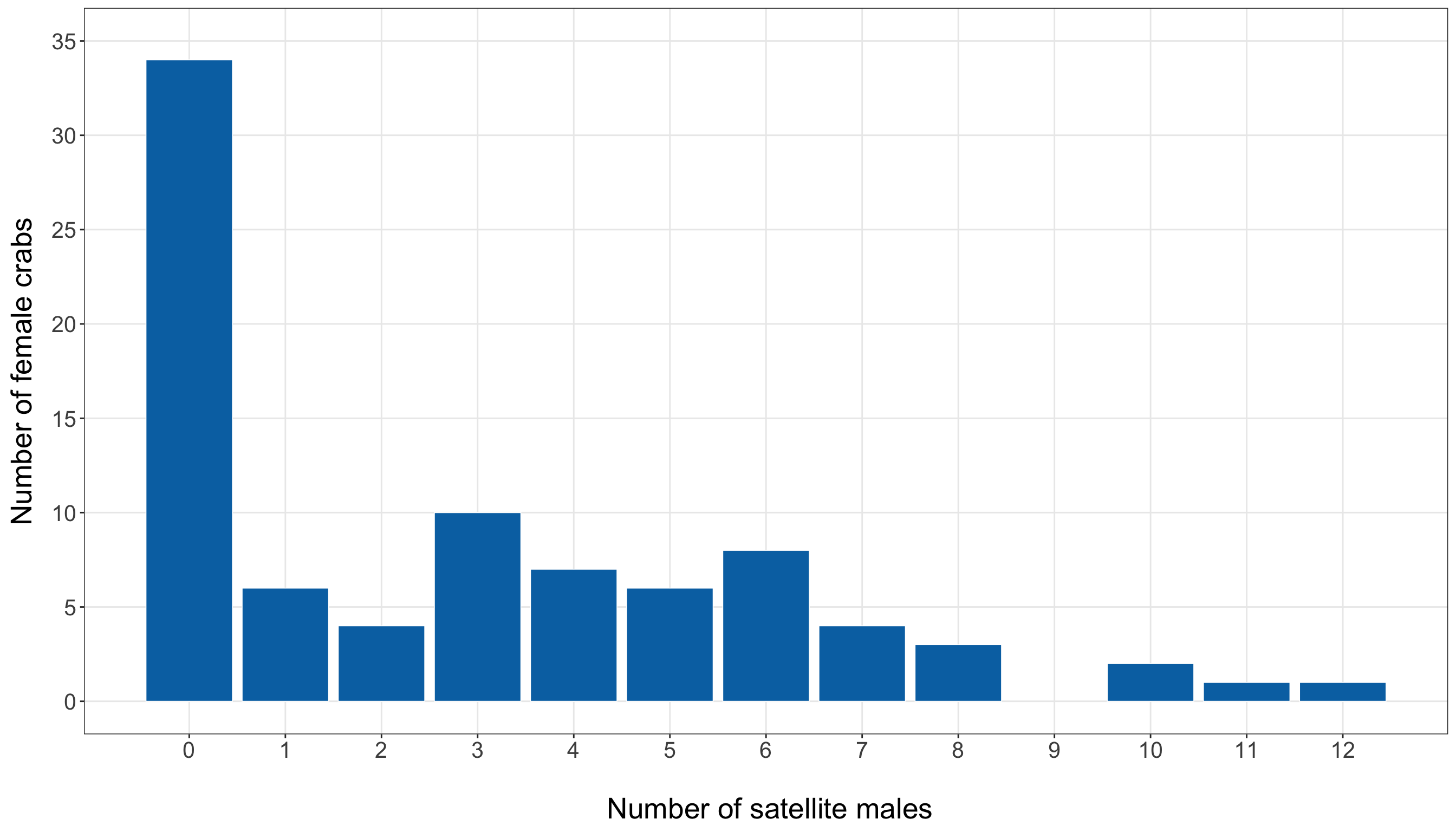
# Importing library
import matplotlib.pyplot as plt

satellite_counts = (
    training_data["satellites"]
    .value_counts()
    .sort_index()
)

response_distribution_figure, response_distribution_axis = plt.subplots(
    figsize=(14, 8)
)

response_distribution_axis.bar(
    satellite_counts.index,
    satellite_counts.values,
    edgecolor="white",
    linewidth=0.3,
    color="#0072B2"
)

response_distribution_axis.set_xlabel(
    "\n Number of satellite males",
    fontsize=20
)

response_distribution_axis.set_ylabel(
    "Number of female crabs",
    fontsize=20,
    labelpad=12
)

response_distribution_axis.tick_params(axis="both", labelsize=15.5)

response_distribution_axis.set_xticks(
    range(
        int(training_data["satellites"].min()),
        int(training_data["satellites"].max()) + 1
    )
)

response_distribution_axis.grid(
    True,
    which="major",
    axis="both",
    alpha=0.3
)

response_distribution_axis.grid(False, which="minor")

response_distribution_figure.tight_layout()
plt.show()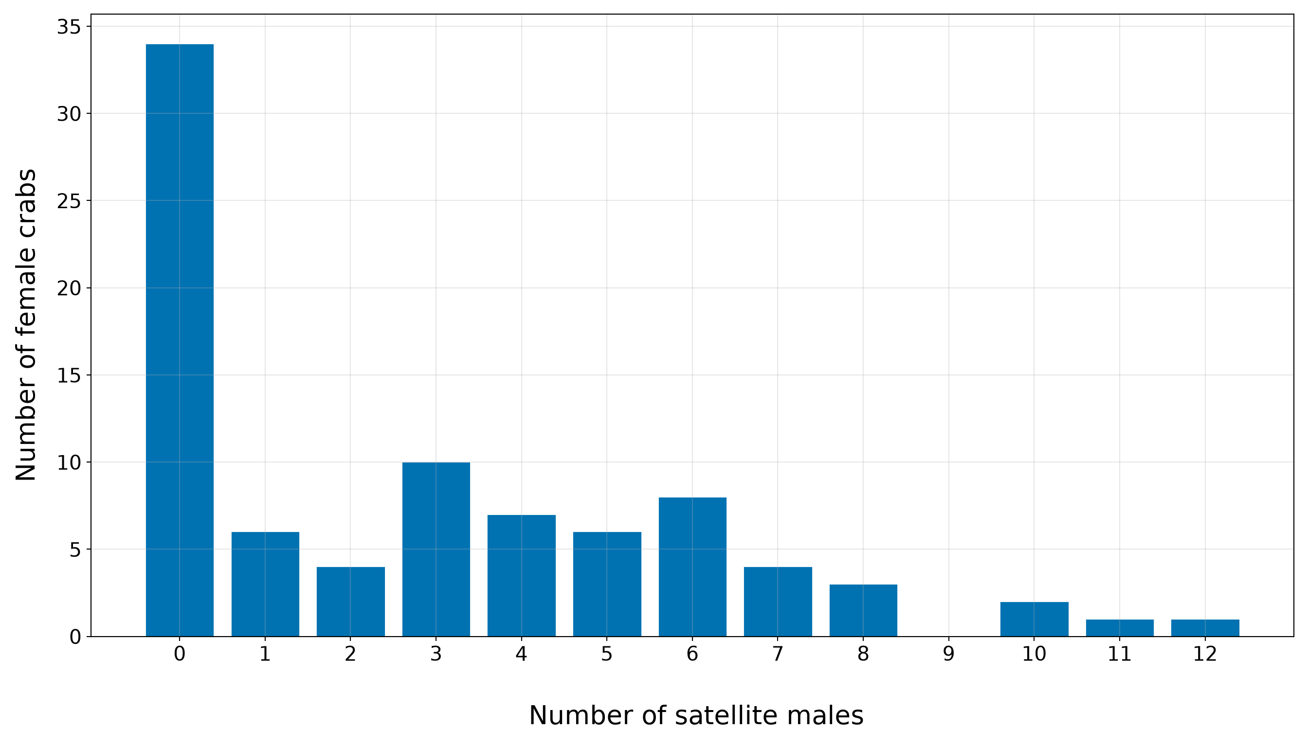
The bar plot confirms that the training-set response is concentrated at zero and relatively small positive counts, with a thinner right tail extending to larger numbers of satellite males. This is critical for the inferential inquiry because the model must describe how the expected count changes with female crab characteristics while respecting the count scale. It is also important for the predictive inquiry because exact observed counts may be difficult to predict: many crabs have no satellites, while a smaller number have much larger counts. Therefore, later predictive results should focus on predicted expected counts and prediction errors, not on pretending that the model can deterministically identify the exact count for each crab.
We have to stress that, at this stage, the above response distribution does not prove that Poisson regression is inappropriate. It tells us what to look for. The large variance relative to the mean suggests possible overdispersion, and the visible number of zeros indicates we should later compare observed and fitted counts carefully. These issues will become part of the goodness-of-fit story before we decide whether the Classical Poisson model is adequate enough for the chapter’s two inquiries.
10.5.3 Satellite Counts and Continuous Regressors

The next part of the EDA examines the response against the two continuous regressors: female crab width and female crab weight. The inferential inquiry asks whether the expected number of satellite males is associated with female crab characteristics, so these plots are the first visual check of whether body size appears relevant. The predictive inquiry also benefits from this step, as a useful predictive model requires regressors that carry information about the response. Hence, we first summarize the response across quartiles of female crab width and weight. These tables are not formal model outputs. They are descriptive summaries that help us read the plots more carefully.
width_quartile_summary <- training_data |>
  mutate(
    width_quartile = ntile(width_cm, 4),
    width_quartile = factor(
      width_quartile,
      levels = 1:4,
      labels = c("Q1: smallest widths", "Q2", "Q3", "Q4: largest widths")
    )
  ) |>
  group_by(width_quartile) |>
  summarise(
    n = n(),
    mean_width_cm = mean(width_cm),
    mean_satellites = mean(satellites),
    median_satellites = median(satellites),
    proportion_zero_satellites = mean(satellites == 0),
    .groups = "drop"
  ) |>
  mutate(
    across(
      where(is.numeric),
      ~ round(.x, 2)
    )
  )

width_quartile_summary |>
  rename(
    `Width quartile` = width_quartile,
    `Number of female crabs` = n,
    `Mean width (cm)` = mean_width_cm,
    `Mean number of satellite males` = mean_satellites,
    `Median number of satellite males` = median_satellites,
    `Proportion with zero satellite males` = proportion_zero_satellites
  ) |>
  kable(
    align = c("c", "c", "c", "c", "c", "c")
)| Width quartile | Number of female crabs | Mean width (cm) | Mean number of satellite males | Median number of satellite males | Proportion with zero satellite males |
|---|---|---|---|---|---|
| Q1: smallest widths | 22 | 23.52 | 1.05 | 0 | 0.68 |
| Q2 | 22 | 25.58 | 2.00 | 0 | 0.55 |
| Q3 | 21 | 26.98 | 3.52 | 3 | 0.19 |
| Q4: largest widths | 21 | 29.38 | 4.95 | 4 | 0.14 |
width_quartile_data = training_data.copy()

width_quartile_data = (
    width_quartile_data
    .sort_values(
        "width_cm",
        kind="mergesort"
    )
    .reset_index(drop=True)
)

number_of_rows = len(width_quartile_data)
number_of_groups = 4

base_group_size = number_of_rows // number_of_groups
remainder = number_of_rows % number_of_groups

group_sizes = [
    base_group_size + 1 if group_index < remainder else base_group_size
    for group_index in range(number_of_groups)
]

quartile_labels = [
    "Q1: smallest widths",
    "Q2",
    "Q3",
    "Q4: largest widths",
]

width_quartile_data["width_quartile"] = np.repeat(
    quartile_labels,
    group_sizes
)

width_quartile_data["width_quartile"] = pd.Categorical(
    width_quartile_data["width_quartile"],
    categories=quartile_labels,
    ordered=True
)

width_quartile_summary = (
    width_quartile_data
    .groupby("width_quartile", observed=False)
    .agg(
        n=("satellites", "size"),
        mean_width_cm=("width_cm", "mean"),
        mean_satellites=("satellites", "mean"),
        median_satellites=("satellites", "median"),
        proportion_zero_satellites=("satellites", lambda x: (x == 0).mean()),
    )
    .reset_index()
    .round(2)
)

width_quartile_summary_display = width_quartile_summary.rename(
    columns={
        "width_quartile": "Width quartile",
        "n": "Number of female crabs",
        "mean_width_cm": "Mean width (cm)",
        "mean_satellites": "Mean number of satellite males",
        "median_satellites": "Median number of satellite males",
        "proportion_zero_satellites": (
            "Proportion with zero satellite males"
        ),
    }
)

classical_poisson_width_quartile_summary_py_html = (
    width_quartile_summary_display.to_html(
        index=False,
        border=0,
    )
)| Width quartile | Number of female crabs | Mean width (cm) | Mean number of satellite males | Median number of satellite males | Proportion with zero satellite males |
|---|---|---|---|---|---|
| Q1: smallest widths | 22 | 23.52 | 1.05 | 0.0 | 0.68 |
| Q2 | 22 | 25.58 | 2.00 | 0.0 | 0.55 |
| Q3 | 21 | 26.98 | 3.52 | 3.0 | 0.19 |
| Q4: largest widths | 21 | 29.38 | 4.95 | 4.0 | 0.14 |
The above width-quartile summary shows a clear positive descriptive pattern between female crab width and the number of satellite males:
- In the smallest-width quartile, female crabs have an average of 1.05 satellite males, with a median of 0.
- In the largest-width quartile, the average increases to 4.95, with a median of 4.
- The middle quartiles also follow the same general ordering: the mean satellite count rises from 2 in Q2 to 3.52 in Q3.
This monotone increase across width quartiles suggests that female crab width is an important body-size regressor to examine first. Now, let us proceed with the width plots.
Heads-up on smoothing and count-response scatterplots!
In both Figure 10.4 (or Figure 10.5), the orange curve is a LOWESS/LOESS smooth. LOWESS stands for locally weighted scatterplot smoothing, and LOESS stands for locally estimated scatterplot smoothing. Both refer to closely related smoothing methods that draw a flexible trend line through a scatterplot by fitting many small local regressions, each using observations close to a given value on the horizontal axis.
In this chapter, we use the LOWESS/LOESS curve only as a visual guide. It is not the Poisson regression model, and we will not interpret it as a fitted statistical model. Its purpose is simply to help us see whether satellite counts tend to be higher for wider female crabs.
Because we show this plot in both R and Python, we make the smoothing settings explicit. Although R’s geom_smooth(method = "loess") and Python’s lowess() from {statsmodels} are based on closely related ideas, their default settings are not identical. To make the two fitted curves visually comparable, we use the same smoothing fraction in both languages and align the local regression structure as closely as possible.

Since satellites is a count response, the points naturally fall on horizontal bands at values such as \(0\), \(1\), \(2\), and so on. These horizontal bands are useful: they remind us that the response is discrete, not continuous. When a continuous regressor such as width_cm is placed on the \(x\)-axis and a count response is placed on the \(y\)-axis, this banded structure is exactly what we should expect.
satellites_width_plot <- ggplot(training_data, aes(x = width_cm, y = satellites)) +
  geom_point(
    alpha = 0.65,
    size = 2.3,
    colour = "#0072B2"
  ) +
  geom_smooth(
    method = "loess",
    formula = y ~ x,
    se = FALSE,
    linewidth = 1.2,
    colour = "#D55E00",
    method.args = list(
      span = 0.75,
      degree = 1,
      family = "gaussian"
    )
  )  +
  theme_bw() +
  theme(
    axis.text = element_text(size = 15.5),
    axis.title.x = element_text(size = 20),
    axis.title.y = element_text(
      size = 20,
      vjust = 0.5,
      margin = margin(r = 12)
    ),
    panel.grid.minor = element_blank()
  ) +
  labs(
    x = "\n Female crab width (cm)",
    y = "Number of satellite males"
  ) +
  scale_x_continuous(breaks = seq(22, 34, by = 2)) +
  scale_y_continuous(breaks = seq(0, 12, by = 2))

satellites_width_plot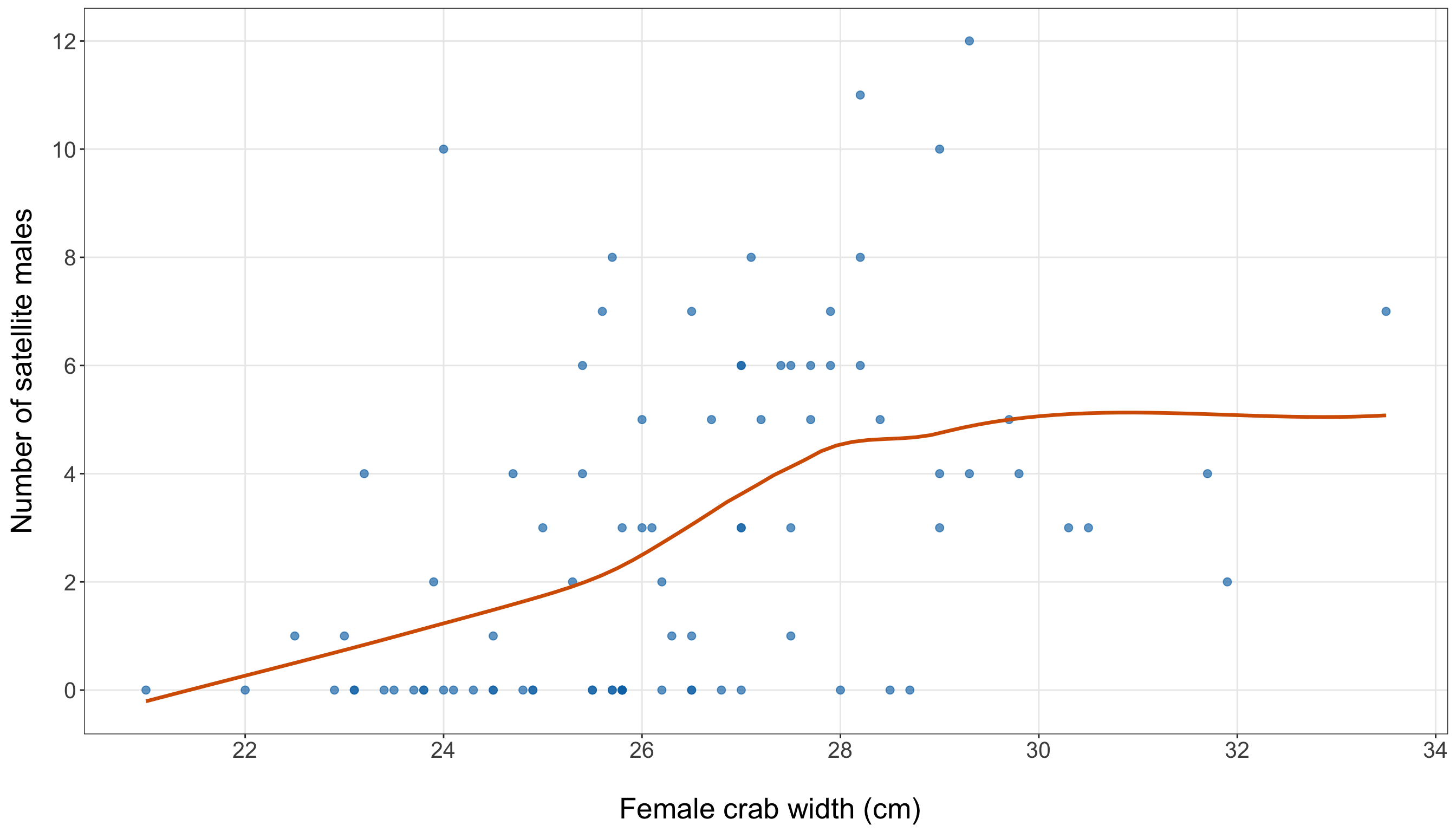
# Importing function
from statsmodels.nonparametric.smoothers_lowess import lowess

width_x = training_data["width_cm"]
sat_y = training_data["satellites"]

smooth_width = lowess(
    endog=sat_y,
    exog=width_x,
    frac=0.75,
    it=0,
    return_sorted=True
)

satellites_width_figure, satellites_width_axis = plt.subplots(
    figsize=(14, 8)
)

satellites_width_axis.scatter(
    width_x,
    sat_y,
    alpha=0.65,
    s=35,
    color="#0072B2"
)

satellites_width_axis.plot(
    smooth_width[:, 0],
    smooth_width[:, 1],
    linewidth=1.2,
    color="#D55E00"
)

satellites_width_axis.set_xlabel(
    "\n Female crab width (cm)",
    fontsize=20
)

satellites_width_axis.set_ylabel(
    "Number of satellite males",
    fontsize=20,
    labelpad=12
)

satellites_width_axis.tick_params(axis="both", labelsize=15.5)
satellites_width_axis.set_xticks(range(22, 35, 2))
satellites_width_axis.set_yticks(range(0, 13, 2))
satellites_width_axis.grid(
    True,
    which="major",
    axis="both",
    alpha=0.3
)

satellites_width_axis.grid(False, which="minor")

satellites_width_figure.tight_layout()
plt.show()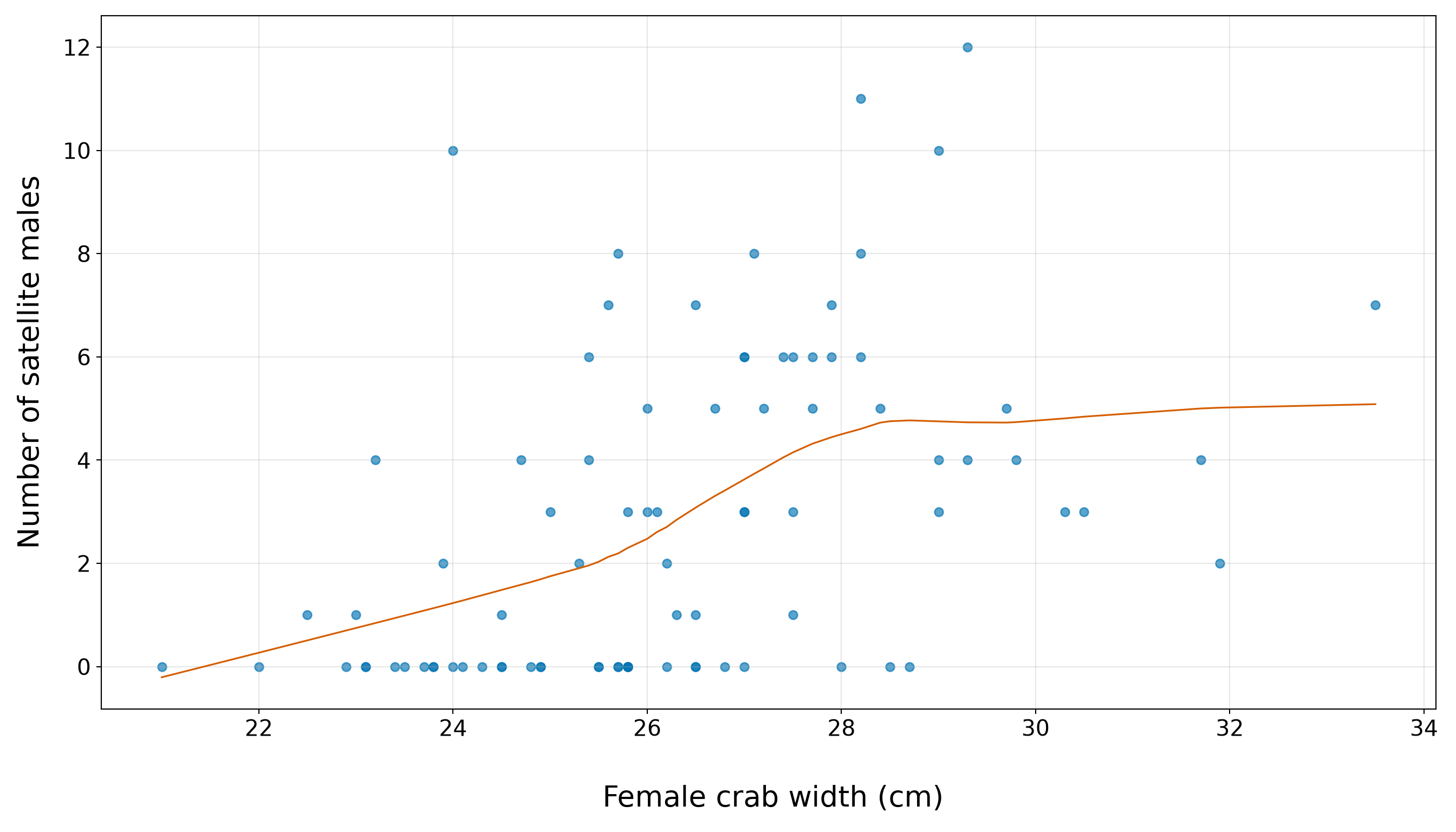
The width plot (from Figure 10.4 or Figure 10.5) should be read together with the quartile (from Table 10.16). The blue points show the observed counts in the training set. Moreover, the orange LOWESS/LOESS curve is only an exploratory visual guide, but it suggests that satellite counts tend to increase as female crab width increases. This agrees with the quartile summary: the average satellite count rises from 1.05 in the smallest-width quartile to 4.95 in the largest-width quartile. Then, the vertical spread around this increasing pattern is also important. Female crabs with similar widths can still have different numbers of satellite males. Some moderate-to-large crabs have zero or very few satellites, while some crabs have much larger counts. This tells us that width is a promising first regressor, but it will not fully explain the response on its own. We will use this EDA result to motivate the first Poisson regression model (see Section 10.7), while leaving formal model specification and interpretation for the next sections.
We now repeat the same EDA logic for female crab weight. Since width and weight both describe body size, we should expect them to tell related but not necessarily identical stories.
weight_quartile_summary <- training_data |>
  mutate(
    weight_quartile = ntile(weight_kg, 4),
    weight_quartile = factor(
      weight_quartile,
      levels = 1:4,
      labels = c("Q1: smallest weights", "Q2", "Q3", "Q4: largest weights")
    )
  ) |>
  group_by(weight_quartile) |>
  summarise(
    n = n(),
    mean_weight_kg = mean(weight_kg),
    mean_satellites = mean(satellites),
    median_satellites = median(satellites),
    proportion_zero_satellites = mean(satellites == 0),
    .groups = "drop"
  ) |>
  mutate(
    across(
      where(is.numeric),
      ~ round(.x, 2)
    )
  )

weight_quartile_summary |>
  rename(
    `Weight quartile` = weight_quartile,
    `Number of female crabs` = n,
    `Mean weight (kg)` = mean_weight_kg,
    `Mean number of satellite males` = mean_satellites,
    `Median number of satellite males` = median_satellites,
    `Proportion with zero satellite males` = proportion_zero_satellites
  ) |>
  kable(
    align = c("c", "c", "c", "c", "c", "c")
)| Weight quartile | Number of female crabs | Mean weight (kg) | Mean number of satellite males | Median number of satellite males | Proportion with zero satellite males |
|---|---|---|---|---|---|
| Q1: smallest weights | 22 | 1.72 | 1.14 | 0 | 0.64 |
| Q2 | 22 | 2.17 | 1.73 | 0 | 0.55 |
| Q3 | 21 | 2.60 | 3.48 | 5 | 0.29 |
| Q4: largest weights | 21 | 3.34 | 5.19 | 4 | 0.10 |
weight_quartile_data = training_data.copy()

weight_quartile_data = (
    weight_quartile_data
    .sort_values(
        "weight_kg",
        kind="mergesort"
    )
    .reset_index(drop=True)
)

number_of_rows = len(weight_quartile_data)
number_of_groups = 4

base_group_size = number_of_rows // number_of_groups
remainder = number_of_rows % number_of_groups

group_sizes = [
    base_group_size + 1 if group_index < remainder else base_group_size
    for group_index in range(number_of_groups)
]

quartile_labels = [
    "Q1: smallest weights",
    "Q2",
    "Q3",
    "Q4: largest weights",
]

weight_quartile_data["weight_quartile"] = np.repeat(
    quartile_labels,
    group_sizes
)

weight_quartile_data["weight_quartile"] = pd.Categorical(
    weight_quartile_data["weight_quartile"],
    categories=quartile_labels,
    ordered=True
)

weight_quartile_summary = (
    weight_quartile_data
    .groupby("weight_quartile", observed=False)
    .agg(
        n=("satellites", "size"),
        mean_weight_kg=("weight_kg", "mean"),
        mean_satellites=("satellites", "mean"),
        median_satellites=("satellites", "median"),
        proportion_zero_satellites=("satellites", lambda x: (x == 0).mean()),
    )
    .reset_index()
    .round(2)
)

weight_quartile_summary_display = weight_quartile_summary.rename(
    columns={
        "weight_quartile": "Weight quartile",
        "n": "Number of female crabs",
        "mean_weight_kg": "Mean weight (kg)",
        "mean_satellites": "Mean number of satellite males",
        "median_satellites": "Median number of satellite males",
        "proportion_zero_satellites": (
            "Proportion with zero satellite males"
        ),
    }
)

classical_poisson_weight_quartile_summary_py_html = (
    weight_quartile_summary_display.to_html(
        index=False,
        border=0,
    )
)| Weight quartile | Number of female crabs | Mean weight (kg) | Mean number of satellite males | Median number of satellite males | Proportion with zero satellite males |
|---|---|---|---|---|---|
| Q1: smallest weights | 22 | 1.72 | 1.14 | 0.0 | 0.64 |
| Q2 | 22 | 2.17 | 1.73 | 0.0 | 0.55 |
| Q3 | 21 | 2.60 | 3.48 | 5.0 | 0.29 |
| Q4: largest weights | 21 | 3.34 | 5.19 | 4.0 | 0.10 |
The weight-quartile summary also points toward a positive body-size pattern:
- In the smallest-weight quartile, the average satellite count is 1.14, with a median of 0.
- In the largest-weight quartile, the average satellite count is 5.19, with a median of 4.
Thus, in the training data, heavier female crabs tend to have higher satellite counts. However, this is still an exploratory pattern, not a biological conclusion. Table 10.18 groups a continuous regressor into four broad bins, and it does not adjust for other female crab characteristics. In particular, the weight summary should be interpreted alongside the width summary, not in isolation. Width and weight are both body-size measurements, so part of the apparent weight pattern may overlap with the width pattern. This is one reason the chapter begins with a simple width-only model before considering an extended model with additional regressors. We will treat weight as a candidate body-size regressor to examine later, while leaving formal interpretation to the fitted regression model.
satellites_weight_plot <- ggplot(
  training_data,
  aes(x = weight_kg, y = satellites)
) +
  geom_point(
    alpha = 0.65,
    size = 2.3,
    colour = "#0072B2"
  ) +
  geom_smooth(
    method = "loess",
    formula = y ~ x,
    se = FALSE,
    linewidth = 1.2,
    colour = "#D55E00",
    method.args = list(
      span = 0.75,
      degree = 1,
      family = "gaussian"
    )
  ) +
  theme_bw() +
  theme(
    axis.text = element_text(size = 15.5),
    axis.title.x = element_text(size = 20),
    axis.title.y = element_text(
      size = 20,
      vjust = 0.5,
      margin = margin(r = 12)
    ),
    panel.grid.minor = element_blank()
  ) +
  labs(
    x = "\n Female crab weight (kg)",
    y = "Number of satellite males"
  ) +
  scale_x_continuous(breaks = seq(1, 5.5, by = 0.5)) +
  scale_y_continuous(breaks = seq(0, 12, by = 2))

satellites_weight_plot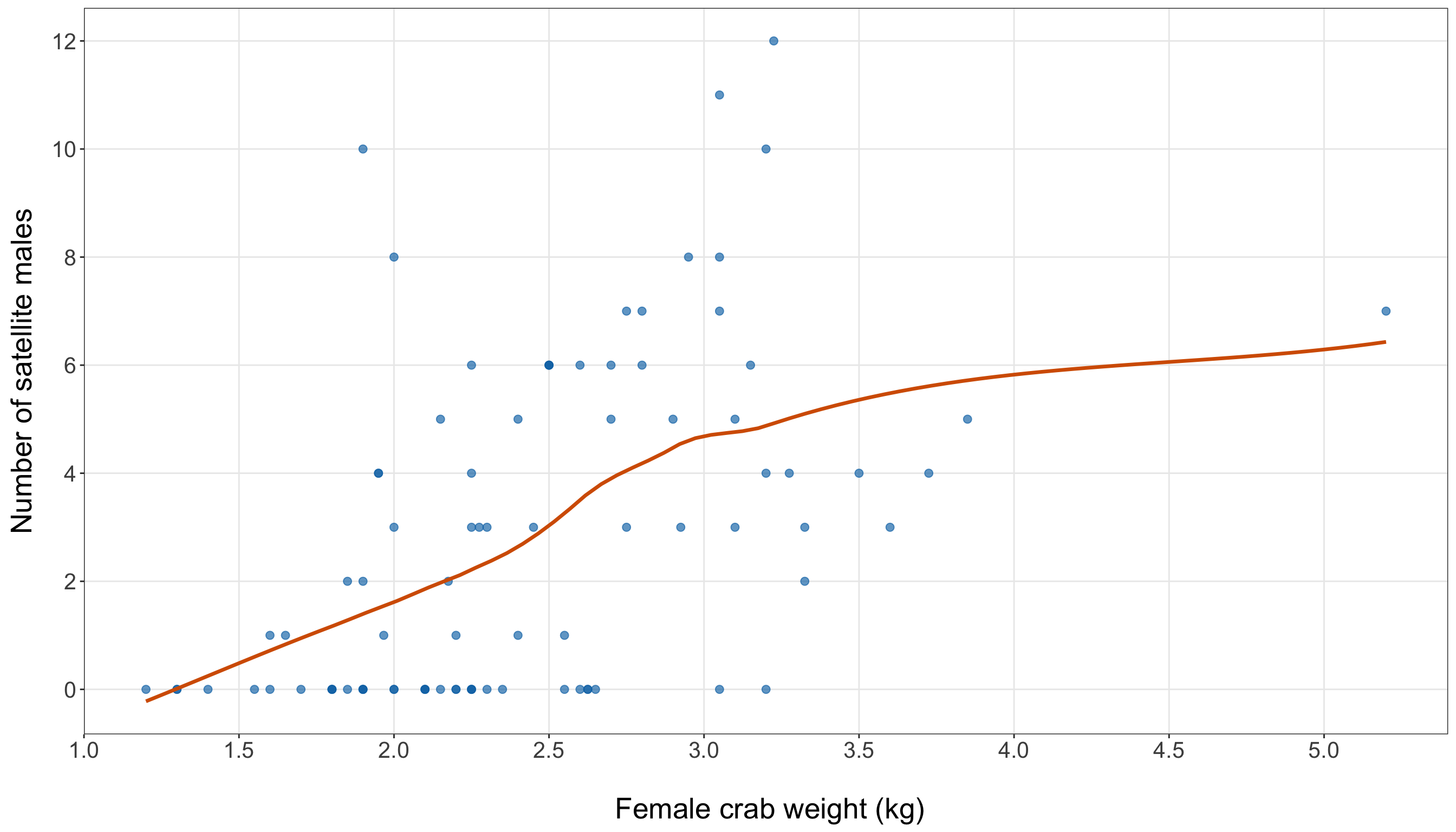
weight_x = training_data["weight_kg"]
sat_y = training_data["satellites"]

smooth_weight = lowess(
    endog=sat_y,
    exog=weight_x,
    frac=0.75,
    it=0,
    return_sorted=True
)

satellites_weight_figure, satellites_weight_axis = plt.subplots(
    figsize=(14, 8)
)

satellites_weight_axis.scatter(
    weight_x,
    sat_y,
    alpha=0.65,
    s=35,
    color="#0072B2"
)

satellites_weight_axis.plot(
    smooth_weight[:, 0],
    smooth_weight[:, 1],
    linewidth=1.2,
    color="#D55E00"
)

satellites_weight_axis.set_xlabel(
    "\n Female crab weight (kg)",
    fontsize=20
)

satellites_weight_axis.set_ylabel(
    "Number of satellite males",
    fontsize=20,
    labelpad=12
)

satellites_weight_axis.tick_params(axis="both", labelsize=15.5)
satellites_weight_axis.set_xticks(np.arange(1, 5.6, 0.5))
satellites_weight_axis.set_yticks(range(0, 13, 2))

satellites_weight_axis.grid(
    True,
    which="major",
    axis="both",
    alpha=0.3
)

satellites_weight_axis.grid(False, which="minor")

satellites_weight_figure.tight_layout()
plt.show()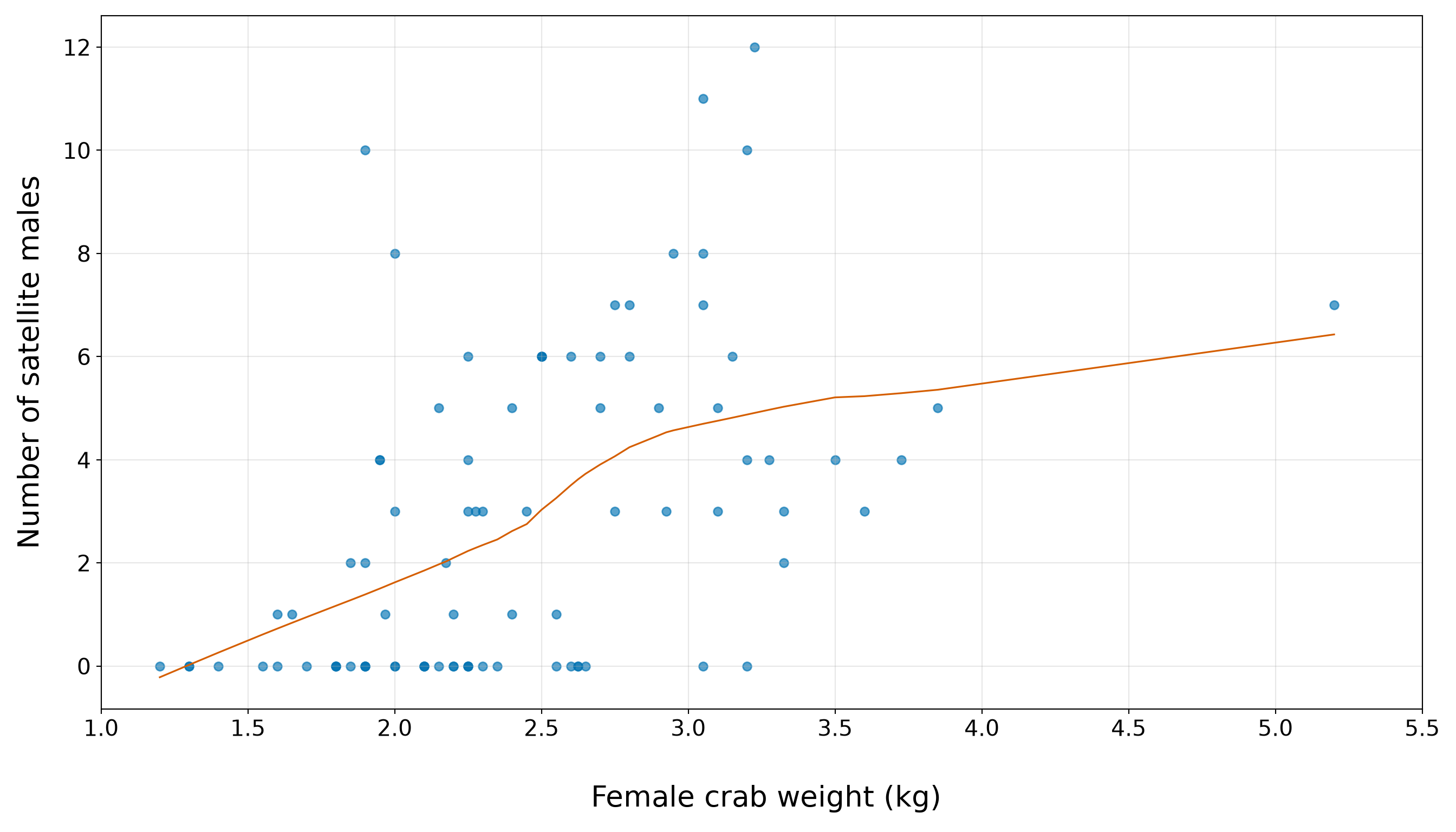
The weight plot, in Figure 10.6 or Figure 10.7, should be read with the same caution as the width plot. The horizontal bands again show that the response is a count, not a continuous outcome. The orange smooth gives an exploratory body-size trend, and the quartile table gives the corresponding numerical summary. The main EDA message is that heavier female crabs tend to have higher satellite counts, but the relationship is not deterministic. There are still zero counts and small positive counts across much of the weight range. Therefore, weight may add useful information in an extended model, but it should not be treated as a complete explanation of satellite counts.
10.5.4 Satellite Counts and Categorical Regressors

Now, we compare satellite counts across the categorical regressors color and spine. Earlier, in Section 10.5.1, the marginal summaries showed that these categories are not evenly represented in the training data. That imbalance is critical here because a category with few observations can have an unstable mean satellite count. Therefore, in this subsection, we combine two pieces of information: the number of observations in each category and the distribution of satellite counts within each category.
We begin with female crab colour.
color_satellite_summary <- training_data |>
  group_by(color) |>
  summarise(
    n = n(),
    mean_satellites = mean(satellites),
    median_satellites = median(satellites),
    proportion_zero_satellites = mean(satellites == 0),
    .groups = "drop"
  ) |>
  mutate(
    across(
      where(is.numeric),
      ~ round(.x, 2)
    )
  )

color_satellite_summary |>
  rename(
    `Female crab colour` = color,
    `Number of female crabs` = n,
    `Mean number of satellite males` = mean_satellites,
    `Median number of satellite males` = median_satellites,
    `Proportion with zero satellite males` = proportion_zero_satellites
  ) |>
  kable(
    align = c("c", "c", "c", "c", "c")
)| Female crab colour | Number of female crabs | Mean number of satellite males | Median number of satellite males | Proportion with zero satellite males |
|---|---|---|---|---|
| Light | 8 | 3.38 | 3.5 | 0.38 |
| Medium light | 44 | 3.34 | 3.0 | 0.32 |
| Medium dark | 22 | 2.41 | 1.5 | 0.36 |
| Dark | 12 | 1.50 | 0.0 | 0.75 |
color_satellite_summary = (
    training_data
    .groupby("color", observed=False)
    .agg(
        n=("satellites", "size"),
        mean_satellites=("satellites", "mean"),
        median_satellites=("satellites", "median"),
        proportion_zero_satellites=("satellites", lambda x: (x == 0).mean()),
    )
    .reset_index()
    .round(2)
)

color_satellite_summary_display = color_satellite_summary.rename(
    columns={
        "color": "Female crab colour",
        "n": "Number of female crabs",
        "mean_satellites": "Mean number of satellite males",
        "median_satellites": "Median number of satellite males",
        "proportion_zero_satellites": (
            "Proportion with zero satellite males"
        ),
    }
)

classical_poisson_color_satellite_summary_py_html = (
    color_satellite_summary_display.to_html(
        index=False,
        border=0,
    )
)| Female crab colour | Number of female crabs | Mean number of satellite males | Median number of satellite males | Proportion with zero satellite males |
|---|---|---|---|---|
| Light | 8 | 3.38 | 3.5 | 0.38 |
| Medium light | 44 | 3.34 | 3.0 | 0.32 |
| Medium dark | 22 | 2.41 | 1.5 | 0.36 |
| Dark | 12 | 1.50 | 0.0 | 0.75 |
The colour summary, in Table 10.20, must be read in light of the category sizes reported earlier. In this training split, the most common colour category is Medium light, while Light and Dark are much less common. The satellite-count summaries suggest that colour may be associated with the response, but the evidence is uneven across categories. The category with the highest mean satellite count is Light, with a mean of 3.38. The category with the lowest mean satellite count is Dark, with a mean of 1.5. These are descriptive differences only. Because some colour categories are sparse, the extended model should treat colour comparisons cautiously.
Heads-up on horizontal jitter in categorical plots!
In the subsequent plots, the orange points are slightly jittered horizontally within each female crab category. This means that points are moved a little to the left or right so that overlapping observations are easier to see. Note that this horizontal jitter is only a plotting device. It does not change the observed number of satellite males. The vertical positions of the points remain the original count values, so the horizontal bands at \(0\), \(1\), \(2\), and so on are preserved. These bands are still important because they remind us that satellites is a count response.

We use a seed in the plotting code so that the small left-right movements are reproducible. In other words, the same code produces the same visual arrangement each time the chapter is rendered.
set.seed(123)

satellites_color_plot <- ggplot(
  training_data,
  aes(x = color, y = satellites)
) +
  geom_boxplot(
    fill = "#0072B2",
    alpha = 0.45,
    outlier.shape = NA
  ) +
  geom_point(
    position = position_jitter(
      width = 0.18,
      height = 0,
      seed = 123
    ),
    alpha = 0.65,
    size = 2.2,
    colour = "#D55E00"
  ) +
  theme_bw() +
  theme(
    axis.text = element_text(size = 15.5),
    axis.title.x = element_text(size = 20),
    axis.title.y = element_text(
      size = 20,
      vjust = 0.5,
      margin = margin(r = 12)
    ),
    panel.grid.minor = element_blank()
  ) +
  labs(
    x = "\n Female crab colour",
    y = "Number of satellite males"
  ) +
  scale_y_continuous(breaks = seq(0, 12, by = 2))

satellites_color_plot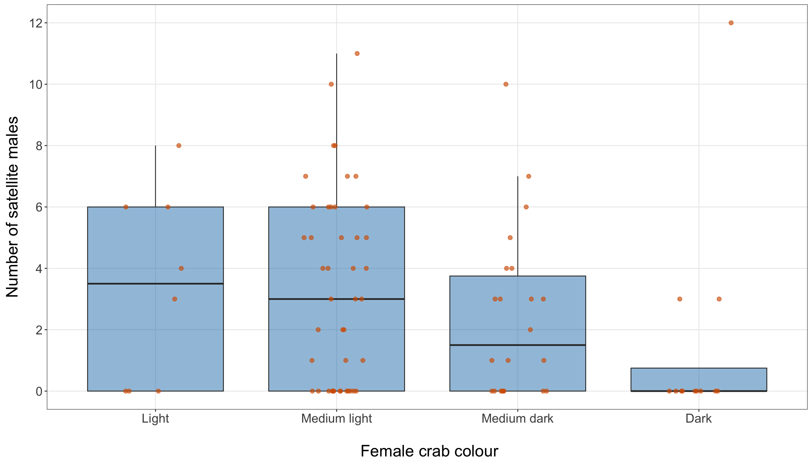
rng = np.random.default_rng(123)

color_order = [
    category
    for category in ["Light", "Medium light", "Medium dark", "Dark"]
    if category in list(training_data["color"].astype(str).unique())
]

color_data = [
    training_data.loc[
        training_data["color"].astype(str) == category,
        "satellites"
    ].to_numpy()
    for category in color_order
]

satellites_color_figure, satellites_color_axis = plt.subplots(
    figsize=(14, 8)
)

color_box = satellites_color_axis.boxplot(
    color_data,
    tick_labels=color_order,
    patch_artist=True,
    showfliers=False
)

for patch in color_box["boxes"]:
    patch.set_facecolor("#0072B2")
    patch.set_alpha(0.45)

for index, category in enumerate(color_order, start=1):
    y_values = training_data.loc[
        training_data["color"].astype(str) == category,
        "satellites"
    ].to_numpy()

    x_values = index + rng.uniform(
        -0.18,
        0.18,
        size=len(y_values)
    )

    satellites_color_axis.scatter(
        x_values,
        y_values,
        alpha=0.65,
        s=30,
        color="#D55E00"
    )

satellites_color_axis.set_xlabel(
    "\n Female crab colour",
    fontsize=20
)

satellites_color_axis.set_ylabel(
    "Number of satellite males",
    fontsize=20,
    labelpad=12
)

satellites_color_axis.tick_params(axis="both", labelsize=15.5)
satellites_color_axis.set_yticks(range(0, 13, 2))

satellites_color_axis.grid(
    True,
    which="major",
    axis="both",
    alpha=0.3
)

satellites_color_axis.grid(False, which="minor")

satellites_color_figure.tight_layout()
plt.show()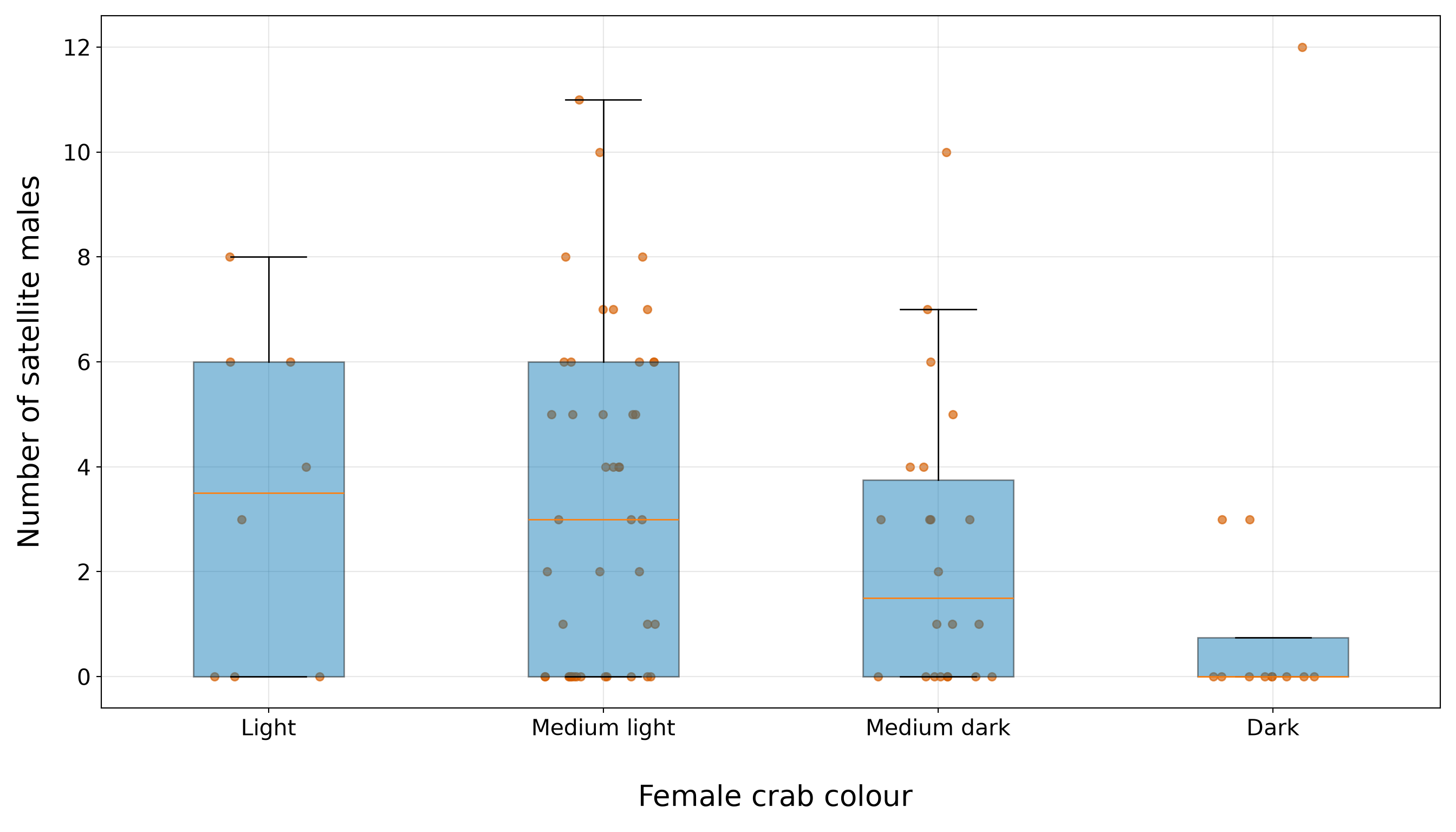
The colour plot, in Figure 10.8 or Figure 10.9, reinforces the table’s cautionary message. The boxplots and horizontally jittered points show substantial overlap in satellite counts across colour categories. This means colour may still be useful in an extended model, but it is unlikely to separate the response cleanly on its own. The horizontal jitter is used only to reduce overlap within each colour category; it does not move the counts vertically, so the integer count bands remain visible.
We now repeat the same comparison for female crab spine condition.
spine_satellite_summary <- training_data |>
  group_by(spine) |>
  summarise(
    n = n(),
    mean_satellites = mean(satellites),
    median_satellites = median(satellites),
    proportion_zero_satellites = mean(satellites == 0),
    .groups = "drop"
  ) |>
  mutate(
    across(
      where(is.numeric),
      ~ round(.x, 2)
    )
  )

spine_satellite_summary |>
  rename(
    `Female crab spine condition` = spine,
    `Number of female crabs` = n,
    `Mean number of satellite males` = mean_satellites,
    `Median number of satellite males` = median_satellites,
    `Proportion with zero satellite males` = proportion_zero_satellites
  ) |>
  kable(
    align = c("c", "c", "c", "c", "c")
)| Female crab spine condition | Number of female crabs | Mean number of satellite males | Median number of satellite males | Proportion with zero satellite males |
|---|---|---|---|---|
| Both good | 20 | 3.25 | 3.5 | 0.35 |
| One worn or broken | 7 | 1.57 | 0.0 | 0.57 |
| Both worn or broken | 59 | 2.86 | 2.0 | 0.39 |
spine_satellite_summary = (
    training_data
    .groupby("spine", observed=False)
    .agg(
        n=("satellites", "size"),
        mean_satellites=("satellites", "mean"),
        median_satellites=("satellites", "median"),
        proportion_zero_satellites=("satellites", lambda x: (x == 0).mean()),
    )
    .reset_index()
    .round(2)
)

spine_satellite_summary_display = spine_satellite_summary.rename(
    columns={
        "spine": "Female crab spine condition",
        "n": "Number of female crabs",
        "mean_satellites": "Mean number of satellite males",
        "median_satellites": "Median number of satellite males",
        "proportion_zero_satellites": (
            "Proportion with zero satellite males"
        ),
    }
)

classical_poisson_spine_satellite_summary_py_html = (
    spine_satellite_summary_display.to_html(
        index=False,
        border=0,
    )
)| Female crab spine condition | Number of female crabs | Mean number of satellite males | Median number of satellite males | Proportion with zero satellite males |
|---|---|---|---|---|
| Both good | 20 | 3.25 | 3.5 | 0.35 |
| One worn or broken | 7 | 1.57 | 0.0 | 0.57 |
| Both worn or broken | 59 | 2.86 | 2.0 | 0.39 |
The spine summary, in Table 10.22, is dominated by the Both worn or broken category, which was already the largest group in the marginal spine table. This imbalance is important. The category with the highest mean satellite count is Both good, with a mean of 3.25. The category with the lowest mean satellite count is One worn or broken, with a mean of 1.57. However, because at least one spine category has relatively few observations, these descriptive differences should not be over-interpreted before modelling.
set.seed(123)

satellites_spine_plot <- ggplot(
  training_data,
  aes(x = spine, y = satellites)
) +
  geom_boxplot(
    fill = "#0072B2",
    alpha = 0.45,
    outlier.shape = NA
  ) +
  geom_point(
    position = position_jitter(
      width = 0.18,
      height = 0,
      seed = 123
    ),
    alpha = 0.65,
    size = 2.2,
    colour = "#D55E00"
  ) +
  theme_bw() +
  theme(
    axis.text = element_text(size = 15.5),
    axis.title.x = element_text(size = 20),
    axis.title.y = element_text(
      size = 20,
      vjust = 0.5,
      margin = margin(r = 12)
    ),
    panel.grid.minor = element_blank()
  ) +
  labs(
    x = "\n Female crab spine condition",
    y = "Number of satellite males"
  ) +
  scale_y_continuous(breaks = seq(0, 12, by = 2))

satellites_spine_plot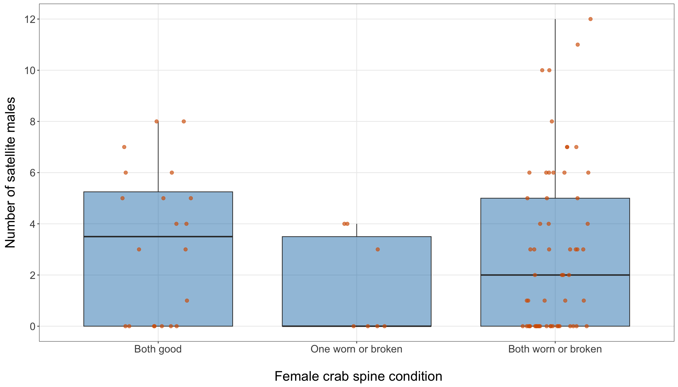
spine_order = [
    category
    for category in [
        "Both good",
        "One worn or broken",
        "Both worn or broken",
    ]
    if category in list(training_data["spine"].astype(str).unique())
]

spine_data = [
    training_data.loc[
        training_data["spine"].astype(str) == category,
        "satellites"
    ].to_numpy()
    for category in spine_order
]

satellites_spine_figure, satellites_spine_axis = plt.subplots(
    figsize=(14, 8)
)

spine_box = satellites_spine_axis.boxplot(
    spine_data,
    tick_labels=spine_order,
    patch_artist=True,
    showfliers=False
)

for patch in spine_box["boxes"]:
    patch.set_facecolor("#0072B2")
    patch.set_alpha(0.45)

for index, category in enumerate(spine_order, start=1):
    y_values = training_data.loc[
        training_data["spine"].astype(str) == category,
        "satellites"
    ].to_numpy()

    x_values = index + rng.uniform(
        -0.18,
        0.18,
        size=len(y_values)
    )

    satellites_spine_axis.scatter(
        x_values,
        y_values,
        alpha=0.65,
        s=30,
        color="#D55E00"
    )

satellites_spine_axis.set_xlabel(
    "\n Female crab spine condition",
    fontsize=20
)

satellites_spine_axis.set_ylabel(
    "Number of satellite males",
    fontsize=20,
    labelpad=12
)

satellites_spine_axis.tick_params(axis="both", labelsize=15.5)
satellites_spine_axis.set_yticks(range(0, 13, 2))

satellites_spine_axis.grid(
    True,
    which="major",
    axis="both",
    alpha=0.3
)

satellites_spine_axis.grid(False, which="minor")

satellites_spine_figure.tight_layout()
plt.show()
The spine plot, in Figure 10.10 or Figure 10.11, again shows overlap across categories. The largest category contains crabs with a wide range of satellite counts, including zero counts and larger positive counts. The smaller categories are harder to compare because they contain fewer observations. This makes spine a reasonable candidate regressor for the extended model, but not one that should be expected to dominate the body-size pattern seen for width and weight.
10.5.5 Summary

Before moving to the GLM formulation of Poisson regression, it is useful to summarize the main EDA findings. Table 10.24 records what we learned from the training data and how each finding will guide the next parts of the workflow.
| EDA component | Main finding from the training data | Why it matters for the Poisson regression workflow |
|---|---|---|
| Response distribution | The response satellites is a non-negative integer count. The training data contain 34 zero counts out of 86 observations. The mean number of satellite males is 2.85, while the variance is 9.61, giving a variance-to-mean ratio of 3.37. |
Poisson regression is a natural starting point because the response is a count. However, the variance is much larger than the mean, so the Classical Poisson mean-variance structure will need to be checked carefully later. |
| Count-response plot | The bar plot shows many zero and small positive counts, with a thinner right tail extending to larger satellite counts. | This reinforces that we are modelling a discrete, right-skewed count response. The large counts and the visible number of zeros motivate later observed-versus-fitted checks. |
| Width and satellite counts | The width-quartile summary shows a clear positive descriptive pattern: the mean satellite count rises from 1.05 in the smallest-width quartile to 4.95 in the largest-width quartile. The width scatterplot shows the same general upward pattern, while preserving the horizontal bands created by the count response. | Width has the clearest descriptive body-size pattern in the EDA, so it is a sensible first regressor for the simple Poisson regression model. The vertical spread at similar widths also warns us that width alone will not fully explain the response. |
| Weight and satellite counts | The weight-quartile summary also suggests a positive descriptive association: the mean satellite count changes from 1.14 in the smallest-weight quartile to 5.19 in the largest-weight quartile. The weight plot shows a related body-size pattern, again with substantial variability around the visual trend. | Weight is a candidate body-size regressor for the extended model. However, width and weight should not be interpreted in isolation because they both describe body size and may partly carry overlapping information. |
| Female crab colour | Colour groups have uneven sample sizes. The category with the highest mean satellite count is Light, with a mean of 3.38. The category with the lowest mean satellite count is Dark, with a mean of 1.5. |
Colour may be useful in the extended model, but category-level comparisons should be treated cautiously because some colour groups are sparse and the boxplots show overlap across categories. |
| Female crab spine condition | Spine groups are also imbalanced. The category with the highest mean satellite count is Both good, with a mean of 3.25. The category with the lowest mean satellite count is One worn or broken, with a mean of 1.57. |
Spine condition is worth checking in the extended model, but the EDA does not suggest that it should dominate the body-size regressors. The imbalance across spine categories also means coefficient-level interpretations should be cautious. |
| Predictive challenge | Across the continuous and categorical plots, female crabs with similar regressor values can still have quite different satellite counts. Zero counts also occur across multiple regions of the regressor space. | The predictive inquiry should be evaluated with held-out testing data and prediction-error summaries. Visual patterns from the training data can motivate model choices, but they are not enough to assess predictive performance. |
Overall, the EDA gives us a coherent modelling story. The response is a non-negative integer count with many zeros and variability that is much larger than the mean. Width shows the clearest descriptive association with satellite counts, while weight provides a related body-size signal that should be interpreted alongside width. Colour and spine condition may also contribute, but their category imbalance and overlapping count distributions call for caution. These findings do not establish final inferential conclusions; rather, they motivate the model-building sequence that follows. We now move to the GLM formulation so that the response distribution, regression structure, and coefficient interpretation are made explicit before estimation.
10.6 Poisson Regression as a Generalized Linear Model
In Section 10.5, the EDA indicated that the response variable satellites is a non-negative integer count. This finding is the first reason why Classical Poisson regression serves as a baseline count-based model for this study. However, the EDA also revealed that the response has many zero counts along with a sample variance much larger than its sample mean. While these characteristics do not prevent us from fitting a Poisson regression model, they highlight what we will need to check after fitting it.
Classical Poisson regression is a GLM with three parts:
- a random component, which describes the probability distribution of the response;
- a systematic component, which combines the regressors into a linear expression;
- a link function, which connects the conditional mean of the response to the systematic component.
This structure is different from the OLS model from Chapter 3. In the OLS setup, we commonly write the response as a systematic part plus an additive random error term. For example, with \(k\) regressors,
\[ Y_i = \underbrace{\beta_0 + \beta_1 x_{i,1} + \cdots + \beta_k x_{i, k}}_{\text{Systematic Component}} + \underbrace{\varepsilon_i.}_{\substack{\text{Random} \\ \text{Component}}} \tag{10.1}\]
In Equation 10.1, the systematic component is the linear expression \(\beta_0 + \beta_1 x_{i,1} + \cdots + \beta_k x_{i,k}\), and the random component is often represented by the error term \(\varepsilon_i\). Under the usual classical OLS assumptions, that error term has the following assumptions:
\[ \begin{gather*} \mathbb{E}(\varepsilon_i) = 0 \\ \text{Var}(\varepsilon_i) = \sigma^2 \\ \varepsilon_i \sim \operatorname{Normal}(0, \sigma^2) \\ \varepsilon_i \perp \!\!\! \perp \varepsilon_k \; \; \; \; \text{for} \; i \neq k \; \; \; \; \text{(independence)}. \end{gather*} \]
On the other hand, for Poisson regression, we do not build the model by adding a separate error term to a linear expression. Instead, we model the conditional distribution of the count response directly. The response variable is random, and its conditional mean is a linear function of the regressors. This difference is the main reason why we sometimes find GLMs less familiar than OLS: the systematic component still looks linear, but it is no longer the conditional mean on the original response scale.
Heads-up on comparing OLS and Poisson regression!
In OLS, it is common to think of the response as
\[ \text{Response} = \text{Systematic Component} + \text{Random Component}. \]
This way of thinking is useful for OLS, but it does not transfer directly to Classical Poisson regression. In Poisson regression, we do not write the count response as a linear expression plus an additive error term (i.e., random component). Instead, we specify a probability distribution for the count response and then model its conditional mean. Therefore, the systematic component in Poisson regression is not directly the expected count. It is a linear expression that becomes connected to the expected count through a link function. This distinction is central to understanding GLMs.
We now define these three components for the horseshoe crab satellite-count case study.
10.6.1 The Random Component
Let \(Y_i\) denote the number of satellite males observed for the \(i\)th female crab in the training data, for \(i = 1, 2, \ldots, n\). We treat \(Y_i\) as a random variable because a different sample of female crabs, or a repeated version of the same observational process, could produce different satellite counts. In Classical Poisson regression, the random component assumes that the conditional distribution of \(Y_i\) is Poisson:
\[ Y_i \mid x_{i,1}, x_{i,2}, \ldots, x_{i,k} \sim \operatorname{Poisson}(\mu_i), \tag{10.2}\]
where \(\mu_i > 0\) is the conditional expected number of satellite males for the \(i\)th female crab. The value of \(\mu_i\) is allowed to change from crab to crab because different crabs can have different regressor values.
Equivalently, for a possible count \(y_i \in \{0, 1, 2, \ldots\}\), the conditional probability mass function (PMF) is
\[ p_Y(y_i;\mu_i) = \Pr(Y_i = y_i \mid x_{i,1}, x_{i,2}, \ldots, x_{i,k}) = \frac{\mu_i^{y_i}\exp(-\mu_i)}{y_i!}. \tag{10.3}\]
The parameter \(\mu_i\) has two roles in the Classical Poisson model:
\[ \mathbb{E}(Y_i \mid x_{i,1}, x_{i,2}, \ldots, x_{i,k}) = \mu_i, \]
and
\[ \operatorname{Var}(Y_i \mid x_{i,1}, x_{i,2}, \ldots, x_{i,k}) = \mu_i. \]
Definition of equidispersion
A count regression model is said to have equidispersion when the conditional variance of the response variable is equal to its conditional mean. In Classical Poisson regression, this means that, after conditioning on the \(k\) regressors, the model assumes
\[ \mu_i = \mathbb{E}(Y_i \mid x_{i,1}, x_{i,2}, \ldots, x_{i,k}) = \operatorname{Var}(Y_i \mid x_{i,1}, x_{i,2}, \ldots, x_{i,k}). \]

Equidispersion is a model assumption about the conditional probability distribution of the response variable. It is not the same as saying that the raw sample mean and raw sample variance of the observed counts must be exactly equal.
This mean-variance equality is a defining feature of the Classical Poisson model. It is also why the EDA result (from Table 10.14) comparing the sample mean and sample variance of satellites is important. The EDA comparison was only marginal and descriptive, while the equidispersion assumption is conditional on the regressors included in the model. Still, the large variance-to-mean gap seen in the EDA gives us a reason to check the fitted model carefully later.
When the observed counts vary more than a fitted Classical Poisson model allows, we call that overdispersion. We will define and diagnose overdispersion more carefully in Section 10.8.2.
Tip on the history of the Poisson distribution!
The Poisson distribution is named after the French mathematician Siméon-Denis Poisson (1781–1840). Poisson worked across mathematics, mechanics, physics, and probability, and the distribution now carrying his name is most commonly associated with modelling counts of events. A major probability work by Poisson was Recherches sur la probabilité des jugements en matière criminelle et en matière civile (Poisson 1837).
For a broader distributional view of the Classical Poisson model, see Section D.4 in the distribution appendix. That appendix presents the PMF, support, mean, and variance of the Classical Poisson distribution before we use it here as the random component of a regression model.
For the horseshoe crab data, the random component says that each observed satellite count is a realization of a Poisson random variable, with its own conditional mean \(\mu_i\). This is different from saying that all crabs have the same expected number of satellite males. The whole purpose of the regression model is to let \(\mu_i\) vary systematically with female crab characteristics such as width, weight, colour, and spine condition.
10.6.2 The Systematic Component
The systematic component describes how the regressors are combined before being linked to the conditional mean. With \(k\) regressors, the systematic component is
\[ \eta_i = \beta_0 + \beta_1 x_{i,1} + \beta_2 x_{i,2} + \cdots + \beta_k x_{i,k}, \tag{10.4}\]
where:
- \(\eta_i\) is called the linear predictor for the \(i\)th female crab;
- \(\beta_0\) is the intercept;
- \(\beta_1, \beta_2, \ldots, \beta_k\) are fixed but unknown regression coefficients;
- \(x_{i,1}, x_{i,2}, \ldots, x_{i,k}\) are the observed regressor values for the \(i\)th female crab.
The term linear predictor can be confusing at first. It means that the regressors are combined linearly in the regression coefficients. Thus, it does not mean that the expected count itself must be a linear function of the regressors on the original count scale.
In the horseshoe crab case study, a simple model may use only female crab width:
\[ \eta_i = \beta_0 + \beta_1 x_{i,1}, \]
where \(x_{i,1}\) represents female crab width in centimetres. An extended model may include additional regressors, such as weight, colour indicators, and spine-condition indicators. In that case, \(k\) is larger and the systematic component includes more terms.
For example, using generic regressor notation, we can write the extended model as
\[ \eta_i = \beta_0 + \beta_1 x_{i,1} + \beta_2 x_{i,2} + \cdots + \beta_k x_{i,k}. \]
This notation deliberately uses \(x_{i,1}, x_{i,2}, \ldots, x_{i,k}\) rather than variable names in the equation. Some of these regressors may be continuous, such as width or weight, while others may be indicator (or dummy) variables created from categorical regressors such as colour or spine condition. We will make the exact model specification explicit when fitting the simple and extended models.
Heads-up on what is systematic in a GLM!
The systematic component in a GLM is the linear predictor \(\eta_i\) (as in Equation 10.4), not the response-scale expected count \(\mu_i\). This is a key difference from the way OLS is often introduced. In OLS with the identity link, the systematic component and the conditional mean are on the same scale. On the other hand, in Classical Poisson regression, the systematic component lives on a transformed scale. Therefore, we will need the link function to connect \(\eta_i\) to \(\mu_i\).
A proper distinction between the random and systematic components in Classical Poisson regression is important for interpretation. If we only look at Equation 10.4, it may appear that we are building an OLS regression model. But the random component in Equation 10.2 says the response is a Poisson count, and the next subsection will show that the expected count is connected to \(\eta_i\) through a log link.
10.6.3 The Log Link Function
The link function connects the conditional mean \(\mu_i\) to the systematic component \(\eta_i\). In Classical Poisson regression, the standard link is the log link:
\[ \log(\mu_i) = \eta_i. \tag{10.5}\]
Combining Equation 10.5 with the systematic component in Equation 10.4 gives
\[ \log(\mu_i) = \beta_0 + \beta_1 x_{i,1} + \beta_2 x_{i,2} + \cdots + \beta_k x_{i,k}. \]
Since the logarithm is applied to \(\mu_i\), we can rewrite the model on the expected-count scale by exponentiating both sides:
\[ \mu_i = \exp\left( \beta_0 + \beta_1 x_{i,1} + \beta_2 x_{i,2} + \cdots + \beta_k x_{i,k} \right). \tag{10.6}\]
This form in Equation 10.6 shows why the log link is useful. The expected count \(\mu_i\) must be positive, and the exponential function always produces a positive value. Thus, the model can use a linear predictor \(\eta_i\) that may be any real number while still producing a valid positive conditional mean. Furthermore, the log link also changes how coefficients are interpreted:
- In OLS, a one-unit increase in a regressor is usually interpreted as an additive change in the conditional mean of the response.
- In Classical Poisson regression with a log link, coefficients are interpreted through multiplicative changes in the expected count after exponentiation.
We will return to this point when interpreting the different fitted coefficients in subsequent sections.
Heads-up on why we do not use an identity link here!
A tempting alternative would be to use an identity link, which would set the conditional mean directly equal to the systematic component:
\[ \mu_i = \beta_0 + \beta_1 x_{i,1} + \beta_2 x_{i,2} + \cdots + \beta_k x_{i,k}. \]
This may look familiar because it resembles the conditional mean structure used in OLS. However, it is usually not a good default choice for Poisson regression. The main issue is that \(\mu_i\) is an expected count, so it must be positive. A linear expression can be negative for some regressor values, which would produce an invalid expected count.
Hence, the log link avoids this problem. It lets the systematic component \(\eta_i\) take any real value, while the expected count
\[ \mu_i = \exp(\eta_i) \]
is always positive. This is one reason the log link is the standard link function for Classical Poisson regression.
Tip on the history of Classical Poisson regression!
The Poisson distribution is much older than the modern GLM framework, but Classical Poisson regression is commonly taught today as a member of the GLM family. The GLM framework was formalized by Nelder and Wedderburn (1972), and it provided a unified way to handle models with different response distributions, including Normal, Binomial, Poisson, and Gamma responses.

From this perspective, Classical Poisson regression combines a Poisson random component with a log link and a linear predictor. The word classical is useful in this book because later chapters consider count models that relax or extend the basic Poisson mean-variance structure, such as overdispersed, generalized, or zero-inflated count models.
Putting the three GLM pieces together, the Classical Poisson regression model with \(k\) regressors is
\[ Y_i \mid x_{i,1}, x_{i,2}, \ldots, x_{i,k} \sim \operatorname{Poisson}(\mu_i), \]
with
\[ \log(\mu_i) = \beta_0 + \beta_1 x_{i,1} + \beta_2 x_{i,2} + \cdots + \beta_k x_{i,k}. \]
Equivalently,
\[ \mu_i = \exp\left( \beta_0 + \beta_1 x_{i,1} + \beta_2 x_{i,2} + \cdots + \beta_k x_{i,k} \right). \]
These equations summarize the model we will fit next:
- The random component tells us that the response is conditionally Poisson.
- The systematic component tells us how the regressors are combined.
- The log link tells us how that linear predictor becomes a positive expected count.
In Section 10.5, the EDA helped us decide that this model is a reasonable starting point, especially because the response is a count and width shows a clear descriptive association with satellite counts (see Figure 10.4 or Figure 10.5). But the EDA also warned us that the Classical Poisson assumptions may be strained. After fitting the model, we will need to examine whether the fitted values reproduce the main features of the observed counts and whether the mean-variance structure is adequate enough for the chapter’s inferential and predictive goals.
10.7 Fitting a Simple Poisson Regression Model
Now, we fit the first Poisson regression model in the chapter. The purpose of this model is deliberately modest: we begin with female crab width as the only regressor because the EDA in Section 10.5 showed the clearest descriptive body-size pattern for width. This simple model gives us a transparent starting point for studying estimation, fitted expected counts, and goodness-of-fit before moving to a richer model with additional regressors.

At this point, we will not provide a full substantive interpretation of the estimate width regression coefficient coming from this model. That interpretation belongs later, after we have checked whether the simple Classical Poisson model is adequate and after we have considered an extended model with additional regressors. This ordering is critical for the workflow of the chapter:
- Use the training data for EDA, model fitting, and goodness-of-fit checks.
- Fit a simple Poisson regression model with width as the only regressor.
- Check whether the fitted model reproduces important features of the observed count response.
- Extend the model if needed by adding other regressors such as weight, colour, and spine condition.
- Save final coefficient-level interpretation for the later modelling sections, after model adequacy has been discussed.
This is necessary for the inferential inquiry. We should not use the same data both to explore the model structure and to produce the final inferential claims. Recall that, for the inferential inquiry, the training set is used for model development and goodness-of-fit assessment. Final inferential outputs will be produced later after the model-building workflow has been completed.
10.7.1 Model Specification
Before fitting the width-only model, we first write the general Classical Poisson regression model with \(k\) regressors. Let
\[ \mathbf{x}_i = \begin{bmatrix} 1 \\ x_{i,1} \\ x_{i,2} \\ \vdots \\ x_{i,k} \end{bmatrix} \]
be the regressor vector for the \(i\)th observation, including the leading \(1\) for the intercept. Then, let
\[ \boldsymbol{\beta} = \begin{bmatrix} \beta_0 \\ \beta_1 \\ \beta_2 \\ \vdots \\ \beta_k \end{bmatrix} \]
be the vector of regression coefficients. The systematic component can then be written compactly as
\[ \eta_i = \mathbf{x}_i^\top \boldsymbol{\beta}, \]
where
\[ \mathbf{x}_i^\top \boldsymbol{\beta} = \beta_0 + \beta_1 x_{i,1} + \beta_2 x_{i,2} + \cdots + \beta_k x_{i,k}. \]
For the full training sample with \(n\) observations, we can collect the response values into
\[ \mathbf{y} = \begin{bmatrix} y_1 \\ y_2 \\ \vdots \\ y_n \end{bmatrix}, \]
and the regressors into the design matrix
\[ \mathbf{X} = \begin{bmatrix} 1 & x_{1,1} & x_{1,2} & \cdots & x_{1,k} \\ 1 & x_{2,1} & x_{2,2} & \cdots & x_{2,k} \\ \vdots & \vdots & \vdots & \ddots & \vdots \\ 1 & x_{n,1} & x_{n,2} & \cdots & x_{n,k} \end{bmatrix}. \]
The \(i\)th row of \(\mathbf{X}\) is \(\mathbf{x}_i^\top\). The vector of systematic scores is
\[ \boldsymbol{\eta} = \mathbf{X}\boldsymbol{\beta}. \]
As indicated in Section 10.6.3, in Classical Poisson regression, the conditional mean for the \(i\)th observation is
\[ \mu_i = \exp(\eta_i) = \exp(\mathbf{x}_i^\top \boldsymbol{\beta}). \]
Thus, the general model with \(k\) regressors is
\[ Y_i \mid \mathbf{x}_i \sim \operatorname{Poisson}(\mu_i), \]
with
\[ \log(\mu_i) = \mathbf{x}_i^\top \boldsymbol{\beta}. \] The width-only model is the special case with one regressor. Let \(x_{i,1}\) denote the female crab width in centimetres for the \(i\)th female crab. The simple model is
\[ Y_i \mid x_{i,1} \sim \operatorname{Poisson}(\mu_i), \]
with
\[ \log(\mu_i) = \beta_0 + \beta_1 x_{i,1}. \tag{10.7}\]
Equivalently,
\[ \mu_i = \exp(\beta_0 + \beta_1 x_{i,1}). \tag{10.8}\]
In Equation 10.7 and Equation 10.8, \(\mu_i\) is the expected number of satellite males for a female crab with width \(x_{i,1}\). The model also assumes
\[ \operatorname{Var}(Y_i \mid x_{i,1}) = \mu_i. \]
Therefore, even this simple model carries the equidispersion assumption. Once width is included, the model assumes that the conditional variance of the satellite count equals the conditional mean for crabs with the same width value. This is stronger than merely saying that the raw sample mean and raw sample variance should be similar. It is a model statement about the distribution of counts after conditioning on width.
Heads-up on why we do not interpret the width coefficient yet!
The simple width-only model is handy because it lets us introduce maximum likelihood estimation in a transparent setting. However, we will not yet use this fitted model to make final claims about the association between female crab width and the expected number of satellite males.
There are two reasons for waiting. First, we still need to check whether the simple Classical Poisson model fits the training data adequately. Second, the EDA suggested that other female crab characteristics, such as weight, colour, and spine condition, may also matter. A width-only coefficient can change once additional regressors are included.

For now, the fitted width coefficient is an estimation output. We will return to substantive coefficient interpretation after the goodness-of-fit checks and the extended model.
10.7.2 Estimation
Classical Poisson regression is estimated by maximum likelihood estimation (MLE). The basic idea is to choose the coefficient vector \(\boldsymbol{\beta}\) that makes the observed training data most compatible with the model. Following up with Equation 10.3, for one observation, the Poisson PMF is
\[ p_Y(y_i;\mu_i) = \frac{\mu_i^{y_i}\exp(-\mu_i)}{y_i!}, \]
where
\[ \mu_i = \exp(\mathbf{x}_i^\top \boldsymbol{\beta}). \]
Assuming the training observations are independent conditional on their regressors, the likelihood function for \(\boldsymbol{\beta}\) is
\[ \mathcal{L}(\boldsymbol{\beta};\mathbf{y}) = \prod_{i=1}^n \frac{ \mu_i^{y_i}\exp(-\mu_i) }{ y_i! }. \tag{10.9}\]
Because products can be hard to work with directly, we usually maximize the log-likelihood. Taking the logarithm of Equation 10.9 gives
\[ \ell(\boldsymbol{\beta};\mathbf{y}) = \sum_{i=1}^n \left[ y_i \log(\mu_i) - \mu_i - \log(y_i!) \right]. \tag{10.10}\]
Using \(\log(\mu_i) = \mathbf{x}_i^\top \boldsymbol{\beta}\) and \(\mu_i = \exp(\mathbf{x}_i^\top \boldsymbol{\beta})\), we can rewrite Equation 10.10 as
\[ \ell(\boldsymbol{\beta};\mathbf{y}) = \sum_{i=1}^n \left[ y_i\mathbf{x}_i^\top \boldsymbol{\beta} - \exp(\mathbf{x}_i^\top \boldsymbol{\beta}) - \log(y_i!) \right]. \tag{10.11}\]
The MLE is the value of \(\boldsymbol{\beta}\) that maximizes this log-likelihood:
\[ \hat{\boldsymbol{\beta}}_{\operatorname{MLE,obs}} = \underset{\boldsymbol{\beta}}{\operatorname{argmax}} \; \ell(\boldsymbol{\beta};\mathbf{y}). \tag{10.12}\]
There is no OLS-style closed-form solution for Equation 10.12. Therefore, software uses iterative numerical algorithms, such as Fisher scoring or Iteratively Reweighted Least Squares (IRLS) (Nelder and Wedderburn 1972), to find the coefficient estimates. The IRLS algorithm starts with an initial guess for the coefficient vector \(\boldsymbol{\beta}\), updates the fitted expected counts, builds a locally weighted least-squares problem, updates the coefficients, and repeats this process until the coefficient estimates stop changing in a meaningful way.
To see the estimating logic without going into matrix calculus, let \(x_{i,j}\) denote the value of the \(j\)th regressor for observation \(i\), with \(x_{i,0}=1\) for the intercept. Since
\[ \mu_i = \exp(\beta_0 + \beta_1 x_{i,1} + \cdots + \beta_k x_{i,k}), \]
the derivative of \(\mu_i\) with respect to \(\beta_j\) is
\[ \frac{\partial \mu_i}{\partial \beta_j} = x_{i,j}\mu_i. \]
Differentiating the log-likelihood in Equation 10.11 with respect to \(\beta_j\) gives the score component
\[ \frac{\partial \ell(\boldsymbol{\beta};\mathbf{y})}{\partial \beta_j} = \sum_{i=1}^n x_{i,j} (y_i - \mu_i), \qquad j = 0, 1, \ldots, k. \]
At the MLE, the score equations are set to zero:
\[ \sum_{i=1}^n x_{i,j} (y_i - \hat{\mu}_i) = 0, \qquad j = 0, 1, \ldots, k, \]
where
\[ \hat{\mu}_i = \exp(\mathbf{x}_i^\top \hat{\boldsymbol{\beta}}_{\operatorname{MLE,obs}}). \]
These equations show that the fitted model balances observed and fitted counts after weighting those differences by each regressor. Equivalently,
\[ \sum_{i=1}^n x_{i,j}y_i = \sum_{i=1}^n x_{i,j}\hat{\mu}_i, \qquad j = 0, 1, \ldots, k. \]
This is more general than the intercept-only intuition. For the intercept, since \(x_{i,0}=1\), the score equation becomes
\[ \sum_{i=1}^n (y_i - \hat{\mu}_i) = 0, \]
so that
\[ \sum_{i=1}^n y_i = \sum_{i=1}^n \hat{\mu}_i. \]
This means that an intercept-only Poisson regression model balances the total observed count and the total fitted expected count. But the other score equations are also necessary. For example, in the simple width-only model, the width score equation is
\[ \sum_{i=1}^n x_{i,1}y_i = \sum_{i=1}^n x_{i,1}\hat{\mu}_i. \]
Thus, the fitted model also balances the observed and fitted counts after multiplying them by female crab width. With more regressors, the same kind of balancing condition holds for each regressor in the model.
IRLS is one way software that solves these score equations. At iteration \(t\), suppose the current regression term estimate is \(\boldsymbol{\beta}^{(t)}\). The algorithm computes
\[ \eta_i^{(t)} = \mathbf{x}_i^\top \boldsymbol{\beta}^{(t)} \]
and
\[ \mu_i^{(t)} = \exp(\eta_i^{(t)}). \]
Then, for the Classical Poisson model with a log link, IRLS constructs a working response
\[ z_i^{(t)} = \eta_i^{(t)} + \frac{y_i - \mu_i^{(t)}}{\mu_i^{(t)}}, \]
and a working weight
\[ w_i^{(t)} = \mu_i^{(t)}. \]
At that iteration, the algorithm solves the weighted least-squares problem
\[ \boldsymbol{\beta}^{(t+1)} = \underset{\boldsymbol{b}}{\operatorname{argmin}} \sum_{i=1}^n w_i^{(t)} \left( z_i^{(t)} - \mathbf{x}_i^\top\boldsymbol{b} \right)^2, \]
where \(\boldsymbol{b}\) is a temporary candidate coefficient vector,
\[ \boldsymbol{b} = \begin{bmatrix} b_0 \\ b_1 \\ \vdots \\ b_k \end{bmatrix}. \]
The notation \(\underset{\boldsymbol{b}}{\operatorname{argmin}}\) means that we search over possible values of \(\boldsymbol{b}\) and choose the vector that makes the weighted sum of squared differences as small as possible. That chosen vector becomes the next coefficient update, \(\boldsymbol{\beta}^{(t+1)}\).
In matrix notation, this update can be written as
\[ \boldsymbol{\beta}^{(t+1)} = \left[ \mathbf{X}^\top \mathbf{W}^{(t)} \mathbf{X} \right]^{-1} \mathbf{X}^\top \mathbf{W}^{(t)} \mathbf{z}^{(t)}, \]
where \(\mathbf{z}^{(t)}\) is the vector of working responses and
\[ \mathbf{W}^{(t)} = \operatorname{diag} \left( \mu_1^{(t)}, \mu_2^{(t)}, \ldots, \mu_n^{(t)} \right) \]
is the diagonal matrix of working weights.
The phrase least-squares in IRLS can be slightly misleading at first. We are not fitting an OLS model to the original count response. Instead, each iteration solves a temporary weighted least-squares problem that approximates the Poisson log-likelihood near the current coefficient values. The target remains the Poisson maximum likelihood estimate.
Heads-up on what IRLS is doing in a nutshell!
IRLS turns the Poisson maximum likelihood problem into a sequence of easier weighted least-squares problems. At each step, the algorithm updates two quantities:
- a working response, which approximates the response on the systematic-score scale;
- a set of working weights, which depend on the current fitted expected counts.

For Classical Poisson regression with a log link, observations with larger current fitted expected counts receive larger working weights because
\[ w_i^{(t)} = \mu_i^{(t)}. \]
These weights come from the same mean-variance structure that defines the Classical Poisson model. This is why estimation, fitted values, Fisher information, and model-based standard errors are all connected to the equidispersion assumption.
The algorithm repeats these updates until convergence. Once it converges, the final coefficient vector is reported as
\[ \hat{\boldsymbol{\beta}}_{\operatorname{MLE,obs}}. \]
The resulting fitted expected counts are
\[ \hat{\mu}_i = \exp(\mathbf{x}_i^\top \hat{\boldsymbol{\beta}}_{\operatorname{MLE,obs}}). \]
These fitted expected counts are the quantities used in the score equations, the goodness-of-fit checks, and the fitted-value summaries that follow.

The second derivative also helps us understand the standard errors produced by the fitted model. For coefficients \(\beta_u\) and \(\beta_v\),
\[ \frac{\partial^2 \ell(\boldsymbol{\beta};\mathbf{y})} {\partial \beta_u \partial \beta_v} = - \sum_{i=1}^n x_{i,u}x_{i,v}\mu_i. \]
The corresponding Fisher information matrix has entries
\[ \mathcal{I}_{u,v}(\boldsymbol{\beta}) = \sum_{i=1}^n x_{i,u}x_{i,v}\mu_i. \]
In matrix notation, this can be written as
\[ \mathcal{I}(\boldsymbol{\beta}) = \mathbf{X}^\top \mathbf{W} \mathbf{X}, \]
where
\[ \mathbf{W} = \operatorname{diag}(\mu_1,\mu_2,\ldots,\mu_n). \]
The fitted model uses the estimated means \(\hat{\mu}_1,\hat{\mu}_2,\ldots,\hat{\mu}_n\) to build the estimated Fisher information,
\[ \mathcal{I}(\hat{\boldsymbol{\beta}}_{\operatorname{MLE,obs}}) = \mathbf{X}^\top \hat{\mathbf{W}} \mathbf{X}, \]
where
\[ \hat{\mathbf{W}} = \operatorname{diag}(\hat{\mu}_1,\hat{\mu}_2,\ldots,\hat{\mu}_n). \]
The approximate covariance matrix of the MLE is then
\[ \widehat{\operatorname{Var}} \left( \hat{\boldsymbol{\beta}}_{\operatorname{MLE,obs}} \right) = \left[ \mathcal{I}(\hat{\boldsymbol{\beta}}_{\operatorname{MLE,obs}}) \right]^{-1}. \]
The standard error for \(\hat{\beta}_j\) is the square root of the corresponding diagonal element of this matrix:
\[ \operatorname{SE}(\hat{\beta}_j) = \sqrt{ \left[ \widehat{\operatorname{Var}} \left( \hat{\boldsymbol{\beta}}_{\operatorname{MLE,obs}} \right) \right]_{j,j} }. \]
Heads-up on equidispersion and model-based standard errors!
The standard errors produced by a Classical Poisson regression model are model-based. They rely on the Poisson mean-variance structure,
\[ \operatorname{Var}(Y_i \mid \mathbf{x}_i) = \mu_i. \]
This is why equidispersion is not just a goodness-of-fit detail. It directly affects uncertainty quantification.
If the observed counts are truly more variable than the Classical Poisson model allows, then the fitted mean pattern may still be informative, but the model-based standard errors can be too small. When standard errors are underestimated, Wald statistics can look too large, confidence intervals can be too narrow, and \(p\)-values can look too optimistic. In hypothesis-testing terms, this makes us more prone to Type I errors: rejecting a null hypothesis too often when it is actually true.
We will diagnose this issue later in Section 10.8.2. This same idea will also motivate later count models, such as Negative Binomial regression, which are designed to handle overdispersed count responses more directly.
The main estimation artifacts produced by a fitted Poisson regression model are summarized in Table 10.25.
| Estimation artifact | What it represents | Why it matters |
|---|---|---|
| \(\hat{\boldsymbol{\beta}}_{\operatorname{MLE,obs}}\) | Estimated regression coefficients | Defines the fitted relationship between regressors and the expected count. |
| \(\hat{\eta}_i = \mathbf{x}_i^\top \hat{\boldsymbol{\beta}}_{\operatorname{MLE,obs}}\) | Fitted systematic score | Intermediate quantity on the link-function scale. |
| \(\hat{\mu}_i = \exp(\hat{\eta}_i)\) | Fitted expected count | Response-scale quantity used for fitted values, prediction, and goodness-of-fit checks. |
| \(\mathcal{I}(\hat{\boldsymbol{\beta}}_{\operatorname{MLE,obs}})\) | Estimated Fisher information | Measures the curvature of the log-likelihood around the MLE. |
| \(\widehat{\operatorname{Var}}(\hat{\boldsymbol{\beta}}_{\operatorname{MLE,obs}})\) | Approximate covariance matrix of the coefficient estimates | Source of model-based standard errors. |
| \(\operatorname{SE}(\hat{\beta}_j)\) | Model-based standard error for coefficient \(j\) | Used later for Wald statistics, confidence intervals, and coefficient-level inference. |
We now fit the simple width-only model to the training data. The fitted model is
\[ Y_i \mid x_{i,1} \sim \operatorname{Poisson}(\mu_i), \]
with
\[ \log(\mu_i) = \beta_0 + \beta_1 x_{i,1}, \]
where \(x_{i,1}\) is female crab width in centimetres.
Note the following:
- In the
Rcode below, theformula = satellites ~ width_cmspecifies the response on the left-hand side and the regressor on the right-hand side. As in previous chapters, functionglm()fits GLMs. The argumentfamily = poisson(link = "log")tellsRto use a Poisson random component with a log link, anddata = training_dataensures that the model is fitted only on the training set. Note that we usetidy()from {broom} for a clean tabular display. - The
Pythoncode uses the analogous {statsmodels} formula interface. The functionsmf.glm()specifies the GLM,formula="satellites ~ width_cm"gives the response-regressor relationship,data=training_dataidentifies the training dataset, andfamily=sm.families.Poisson()specifies the Poisson GLM. The final.fit()call runs the numerical MLE routine and stores the fitted model object.
Table 10.26 gives the MLEs and their model-based standard errors for the intercept and width terms. These are the basic numerical ingredients needed for later inference, but we should not jump directly to substantive interpretation. The next step is to check whether the fitted model is adequate enough to support the chapter’s inferential and predictive goals.
library(broom)

simple_poisson_width_model <- glm(
  formula = satellites ~ width_cm,
  family = poisson(link = "log"),
  data = training_data
)

simple_poisson_width_summary <- tidy(
  simple_poisson_width_model
) |>
  mutate(
    across(
      where(is.numeric),
      ~ round(.x, 3)
    )
  )

simple_poisson_width_summary |>
  rename(
    `Term` = term,
    `Estimate` = estimate,
    `Standard error` = std.error,
    `Wald statistic` = statistic,
    `p-value` = p.value
  ) |>
  kable(
    align = c("c", "c", "c", "c", "c")
)| Term | Estimate | Standard error | Wald statistic | p-value |
|---|---|---|---|---|
| (Intercept) | -4.204 | 0.692 | -6.076 | 0 |
| width_cm | 0.195 | 0.025 | 7.791 | 0 |
import statsmodels.api as sm
import statsmodels.formula.api as smf

simple_poisson_width_model = smf.glm(
    formula="satellites ~ width_cm",
    data=training_data,
    family=sm.families.Poisson()
).fit()

simple_poisson_width_summary = pd.DataFrame(
    {
        "Term": simple_poisson_width_model.params.index,
        "Estimate": simple_poisson_width_model.params.values,
        "Standard error": simple_poisson_width_model.bse.values,
        "Wald statistic": simple_poisson_width_model.tvalues.values,
        "p-value": simple_poisson_width_model.pvalues.values,
    }
)

simple_poisson_width_summary = simple_poisson_width_summary.round(3)

classical_poisson_simple_width_fit_py_html = (
    simple_poisson_width_summary.to_html(
        index=False,
        border=0,
    )
)| Term | Estimate | Standard error | Wald statistic | p-value |
|---|---|---|---|---|
| Intercept | -4.204 | 0.692 | -6.076 | 0.0 |
| width_cm | 0.195 | 0.025 | 7.791 | 0.0 |
Having said that, it will be necessary to store the fitted expected counts, because these will be used in Section 10.8.
simple_poisson_width_fitted <- training_data |>
  mutate(
    fitted_expected_count = fitted(simple_poisson_width_model)
  ) |>
  select(
    satellites,
    width_cm,
    fitted_expected_count
  ) |>
  slice_head(n = 10) |>
  mutate(
    fitted_expected_count = round(fitted_expected_count, 3)
  )

simple_poisson_width_fitted |>
  rename(
    `Observed satellite count` = satellites,
    `Female crab width (cm)` = width_cm,
    `Fitted expected count` = fitted_expected_count
  ) |>
  kable(
    align = c("c", "c", "c")
)| Observed satellite count | Female crab width (cm) | Fitted expected count |
|---|---|---|
| 0 | 23.8 | 1.561 |
| 0 | 21.0 | 0.903 |
| 4 | 29.0 | 4.311 |
| 3 | 30.3 | 5.557 |
| 0 | 22.0 | 1.098 |
| 6 | 27.7 | 3.344 |
| 0 | 27.0 | 2.916 |
| 3 | 26.1 | 2.446 |
| 0 | 23.1 | 1.361 |
| 0 | 24.0 | 1.623 |
simple_poisson_width_fitted = (
    training_data
    .assign(
        fitted_expected_count=simple_poisson_width_model.fittedvalues
    )
    [
        [
            "satellites",
            "width_cm",
            "fitted_expected_count",
        ]
    ]
    .head(10)
    .copy()
)

simple_poisson_width_fitted["fitted_expected_count"] = (
    simple_poisson_width_fitted["fitted_expected_count"].round(3)
)

simple_poisson_width_fitted_display = (
    simple_poisson_width_fitted
    .rename(
        columns={
            "satellites": "Observed satellite count",
            "width_cm": "Female crab width (cm)",
            "fitted_expected_count": "Fitted expected count",
        }
    )
)

classical_poisson_simple_fitted_values_py_html = (
    simple_poisson_width_fitted_display.to_html(
        index=False,
        border=0,
    )
)| Observed satellite count | Female crab width (cm) | Fitted expected count |
|---|---|---|
| 0.0 | 23.8 | 1.561 |
| 0.0 | 21.0 | 0.903 |
| 4.0 | 29.0 | 4.311 |
| 3.0 | 30.3 | 5.557 |
| 0.0 | 22.0 | 1.098 |
| 6.0 | 27.7 | 3.344 |
| 0.0 | 27.0 | 2.916 |
| 3.0 | 26.1 | 2.446 |
| 0.0 | 23.1 | 1.361 |
| 0.0 | 24.0 | 1.623 |
The above fitted expected counts are not rounded counts and should not be forced to be integers. They are estimates of \(\mu_i\), the expected number of satellite males for crabs with the corresponding width values. The observed response remains a count, but the fitted conditional mean is allowed to be fractional. This is the quantity we will compare against the observed counts when checking model adequacy.
Heads-up on decimal expected counts!
A Poisson random variable can only take non-negative integer values:
\[ 0, 1, 2, 3, \ldots \]
However, the Poisson mean \(\mu_i\) does not need to be an integer. It can be any non-negative real number. For example, a fitted expected count such as
\[ \hat{\mu}_i = 2.73 \]
does not mean that the model predicts exactly \(2.73\) satellite males for that crab. Instead, it means that, under the fitted model, the expected number of satellite males for crabs with those regressor values is \(2.73\).
The count outcome itself remains discrete, but the fitted expectation can have decimal places. What cannot happen is a negative fitted expected count. This is one reason the log link is useful in Classical Poisson regression: it keeps
\[ \hat{\mu}_i = \exp(\mathbf{x}_i^\top \hat{\boldsymbol{\beta}}_{\operatorname{MLE,obs}}) \]
strictly positive.
10.8 Checking Goodness of Fit
Once we have fitted the simple width-only Poisson regression model, we move into goodness of fit. This stage asks whether the fitted model behaves in a way that is compatible with the modelling story we wrote down. For the simple Classical Poisson regression model, that story has three main pieces:
- the response is conditionally Poisson;
- the log of the expected count is described by female crab width;
- the conditional mean and conditional variance are equal after conditioning on width.
All checks in this section still use the training data. We are not yet measuring prediction accuracy on the test set. The goal here is diagnostic: we are stress-testing the model we just fitted before using it for final inferential or predictive conclusions. This is not data leakage. Data leakage would occur if we used the testing set to make modelling decisions and then treated it as an untouched assessment set. Here, the training set is where model development, model fitting, and goodness-of-fit checking belong.

Heads-up on training-set diagnostics versus test-set prediction!
The goodness-of-fit checks in this section are based on the training data because the model was fitted on the training data. We use these checks to decide whether the fitted modelling assumptions look plausible enough to continue.
This is different from predictive assessment. Predictive assessment asks how well the model performs on held-out observations that were not used to build or check the model. That comes later, in the results stage. For now, we are still inside the model-building loop of the data science workflow: if the fitted model shows serious diagnostic problems, we may need to return to the modelling stage rather than move directly to final results (see Figure 1.12).
For the simple width-only model, we will look at four diagnostic questions:
- Do the fitted expected counts track the observed counts in a reasonable way?
- Is there evidence that the counts are more variable than the Classical Poisson model allows?
- Does the model understate the number of zero counts?
- Is the residual deviance unusually large relative to its degrees of freedom?
These checks are complementary. A single diagnostic rarely decides everything by itself. Instead, we combine plots, summary tables, formal tests, and the purpose of the analysis to decide whether the simple model is adequate enough to move forward.
10.8.1 Observed versus Fitted Counts
The first check compares the observed satellite counts with the fitted expected counts from the simple width-only model. Note that the fitted expected count for the \(i\)th female crab is
\[ \hat{\mu}_i = \exp(\hat{\beta}_0 + \hat{\beta}_1 x_{i,1}), \]
where \(x_{i,1}\) is female crab width in centimetres.
Definition of fitted expected count
In a fitted Classical Poisson regression model with \(k\) regressors, the fitted expected count for the \(i\)th observation is
\[ \hat{\mu}_i = \exp(\mathbf{x}_i^\top \hat{\boldsymbol{\beta}}_{\operatorname{MLE,obs}}). \]
Here, \(\hat{\mu}_i\) is the fitted expected number of events for the \(i\)th observation, \(\mathbf{x}_i\) is the regressor vector
\[ \mathbf{x}_i^\top = \begin{bmatrix} 1 & x_{i,1} & x_{i,2} & \cdots & x_{i,k} \end{bmatrix}, \]
and \(\hat{\boldsymbol{\beta}}_{\operatorname{MLE,obs}}\) is the vector of maximum likelihood estimates
\[ \hat{\boldsymbol{\beta}}_{\operatorname{MLE,obs}}^\top = \begin{bmatrix} \hat{\beta}_{0,\operatorname{MLE,obs}} & \hat{\beta}_{1,\operatorname{MLE,obs}} & \hat{\beta}_{2,\operatorname{MLE,obs}} & \cdots & \hat{\beta}_{k,\operatorname{MLE,obs}} \end{bmatrix}. \]
Equivalently, in scalar notation,
\[ \hat{\mu}_i = \exp\left( \hat{\beta}_{0,\operatorname{MLE,obs}} + \hat{\beta}_{1,\operatorname{MLE,obs}}x_{i,1} + \hat{\beta}_{2,\operatorname{MLE,obs}}x_{i,2} + \cdots + \hat{\beta}_{k,\operatorname{MLE,obs}}x_{i,k} \right). \]
The fitted expected count estimates the conditional expected value \(\mathbb{E}(Y_i \mid \mathbf{x}_i)\) under the fitted model, where \(Y_i\) is the count response for observation \(i\). The observed response \(y_i\) is a count, but the fitted expected count \(\hat{\mu}_i\) does not need to be an integer.
A useful way to start is to compare the observed counts and fitted expected counts across groups of similar fitted values. This is a descriptive calibration check on the training data.
simple_poisson_gof_data <- training_data |>
  mutate(
    fitted_expected_count = fitted(simple_poisson_width_model),
    pearson_residual = (
      satellites - fitted_expected_count
    ) / sqrt(fitted_expected_count),
    fitted_zero_probability = exp(-fitted_expected_count)
  )

fitted_count_calibration <- simple_poisson_gof_data |>
  mutate(
    fitted_count_quartile = ntile(fitted_expected_count, 4),
    fitted_count_quartile = factor(
      fitted_count_quartile,
      levels = 1:4,
      labels = c(
        "Q1: smallest fitted counts",
        "Q2",
        "Q3",
        "Q4: largest fitted counts"
      )
    )
  ) |>
  group_by(fitted_count_quartile) |>
  summarise(
    n = n(),
    mean_observed_count = mean(satellites),
    mean_fitted_expected_count = mean(fitted_expected_count),
    observed_zero_proportion = mean(satellites == 0),
    mean_fitted_zero_probability = mean(fitted_zero_probability),
    .groups = "drop"
  ) |>
  mutate(
    across(
      where(is.numeric),
      ~ round(.x, 3)
    )
  )

fitted_count_calibration |>
  rename(
    `Fitted-count quartile` = fitted_count_quartile,
    `Number of female crabs` = n,
    `Mean observed count` = mean_observed_count,
    `Mean fitted expected count` = mean_fitted_expected_count,
    `Observed zero proportion` = observed_zero_proportion,
    `Mean fitted zero probability` = mean_fitted_zero_probability
  ) |>
  kable(
    align = c("c", "c", "c", "c", "c", "c")
)| Fitted-count quartile | Number of female crabs | Mean observed count | Mean fitted expected count | Observed zero proportion | Mean fitted zero probability |
|---|---|---|---|---|---|
| Q1: smallest fitted counts | 22 | 1.045 | 1.499 | 0.682 | 0.230 |
| Q2 | 22 | 2.000 | 2.215 | 0.545 | 0.111 |
| Q3 | 21 | 3.524 | 2.917 | 0.190 | 0.056 |
| Q4: largest fitted counts | 21 | 4.952 | 4.859 | 0.143 | 0.015 |
simple_poisson_gof_data = training_data.copy()

simple_poisson_gof_data["fitted_expected_count"] = (
    simple_poisson_width_model.fittedvalues
)

simple_poisson_gof_data["pearson_residual"] = (
    (
        simple_poisson_gof_data["satellites"]
        - simple_poisson_gof_data["fitted_expected_count"]
    )
    / np.sqrt(simple_poisson_gof_data["fitted_expected_count"])
)

simple_poisson_gof_data["fitted_zero_probability"] = np.exp(
    -simple_poisson_gof_data["fitted_expected_count"]
)

simple_poisson_gof_data = (
    simple_poisson_gof_data
    .sort_values(
        "fitted_expected_count",
        kind="mergesort"
    )
    .reset_index(drop=True)
)

number_of_rows = len(simple_poisson_gof_data)
number_of_groups = 4

base_group_size = number_of_rows // number_of_groups
remainder = number_of_rows % number_of_groups

group_sizes = [
    base_group_size + 1 if group_index < remainder else base_group_size
    for group_index in range(number_of_groups)
]

quartile_labels = [
    "Q1: smallest fitted counts",
    "Q2",
    "Q3",
    "Q4: largest fitted counts",
]

simple_poisson_gof_data["fitted_count_quartile"] = np.repeat(
    quartile_labels,
    group_sizes
)

fitted_count_calibration = (
    simple_poisson_gof_data
    .groupby("fitted_count_quartile", observed=False)
    .agg(
        n=("satellites", "size"),
        mean_observed_count=("satellites", "mean"),
        mean_fitted_expected_count=("fitted_expected_count", "mean"),
        observed_zero_proportion=("satellites", lambda x: (x == 0).mean()),
        mean_fitted_zero_probability=("fitted_zero_probability", "mean"),
    )
    .reset_index()
    .round(3)
)

fitted_count_calibration_display = fitted_count_calibration.rename(
    columns={
        "fitted_count_quartile": "Fitted-count quartile",
        "n": "Number of female crabs",
        "mean_observed_count": "Mean observed count",
        "mean_fitted_expected_count": "Mean fitted expected count",
        "observed_zero_proportion": "Observed zero proportion",
        "mean_fitted_zero_probability": "Mean fitted zero probability",
    }
)

classical_poisson_fitted_count_calibration_py_html = (
    fitted_count_calibration_display.to_html(
        index=False,
        border=0,
    )
)| Fitted-count quartile | Number of female crabs | Mean observed count | Mean fitted expected count | Observed zero proportion | Mean fitted zero probability |
|---|---|---|---|---|---|
| Q1: smallest fitted counts | 22 | 1.045 | 1.499 | 0.682 | 0.230 |
| Q2 | 22 | 2.000 | 2.215 | 0.545 | 0.111 |
| Q3 | 21 | 3.524 | 2.917 | 0.190 | 0.056 |
| Q4: largest fitted counts | 21 | 4.952 | 4.859 | 0.143 | 0.015 |
The grouped comparison in Table 10.30 shows that the simple width-only model captures the broad increase in mean satellite counts across fitted-count quartiles, but it does not reproduce all parts of the response distribution equally well. The mean fitted expected count is too high in Q1, where the mean observed count is 1.045 and the mean fitted expected count is 1.499. The mean fitted expected count is too low in Q3, where the mean observed count is 3.524 and the mean fitted expected count is 2.917. In Q4, the two values are much closer: the mean observed count is 4.952, while the mean fitted expected count is 4.859. Thus, the fitted mean pattern is directionally useful but not perfectly calibrated.
Also, the zero-count columns in Table 10.30 show a stronger diagnostic concern. In every fitted-count quartile, the observed zero proportion is larger than the mean fitted zero probability. The discrepancy is especially large in Q1 and Q2. In Q1, the observed zero proportion is 0.682, while the mean fitted zero probability is only 0.23. In Q2, the observed zero proportion is 0.545, while the mean fitted zero probability is only 0.111. This suggests that the simple Classical Poisson model is substantially understating the number of zero satellite counts in the training data.
Heads-up on Pearson residuals and mean fitted zero probabilities!
The goodness-of-fit dataset created above includes two quantities that will be used in different diagnostic checks.
The first quantity is the Pearson residual,
\[ r_i^{(P)} = \frac{y_i - \hat{\mu}_i}{\sqrt{\hat{\mu}_i}}. \tag{10.13}\]
Here, \(y_i\) is the observed satellite count for the \(i\)th female crab, and \(\hat{\mu}_i\) is the fitted expected count from the simple width-only Poisson regression model. The denominator \(\sqrt{\hat{\mu}_i}\) comes from the Classical Poisson mean-variance assumption:
\[ \mu_i = \operatorname{Var}(Y_i \mid \mathbf{x}_i). \]
After fitting the model, we replace \(\mu_i\) with \(\hat{\mu}_i\), so the fitted Poisson standard deviation is \(\sqrt{\hat{\mu}_i}\). Pearson residuals therefore measure how far the observed count is from the fitted expected count in units of the fitted Poisson standard deviation. They will be used later to assess whether the residual variation is larger than the Classical Poisson model expects.
The second quantity is the fitted zero probability,
\[ \Pr(Y_i = 0 \mid \mathbf{x}_i; \hat{\boldsymbol{\beta}}_{\operatorname{MLE,obs}}) = \exp(-\hat{\mu}_i). \]
This comes directly from the Poisson PMF. If \(Y_i \mid \mathbf{x}_i \sim \operatorname{Poisson}(\hat{\mu}_i)\), then the fitted probability of observing zero satellite males for the \(i\)th female crab is \(\exp(-\hat{\mu}_i)\).
In the grouped table, the column called mean fitted zero probability averages these fitted zero probabilities within each fitted-count quartile. It is not the probability of a “mean zero.” Rather, it is the average of the model-implied zero probabilities for the female crabs in that group:
\[ \frac{1}{n_g} \sum_{i \in g} \exp(-\hat{\mu}_i), \]
where \(g\) denotes one fitted-count quartile and \(n_g\) is the number of observations in that quartile.
This average can be compared with the observed zero proportion in the same group,
\[ \frac{1}{n_g} \sum_{i \in g} \mathbb{1}(y_i = 0). \]
If the observed zero proportion is much larger than the mean fitted zero probability, the fitted Poisson model is understating how often zero satellite counts occur.
Now, the same comparison can be viewed graphically in Figure 10.12 (or Figure 10.13). The dashed line is a visual reference where the observed count would equal the fitted expected count. Points above the line correspond to female crabs whose observed satellite count is larger than the model’s fitted expected count. Points below the line correspond to female crabs whose observed satellite count is smaller than the fitted expected count.
observed_fitted_plot <- ggplot(
  simple_poisson_gof_data,
  aes(x = fitted_expected_count, y = satellites)
) +
  geom_point(
    alpha = 0.65,
    size = 2.3,
    colour = "#0072B2"
  ) +
  geom_abline(
    intercept = 0,
    slope = 1,
    linetype = "dashed",
    linewidth = 1,
    colour = "#D55E00"
  ) +
  theme_bw() +
  theme(
    axis.text = element_text(size = 15.5),
    axis.title.x = element_text(size = 20),
    axis.title.y = element_text(
      size = 20,
      vjust = 0.5,
      margin = margin(r = 12)
    ),
    panel.grid.minor = element_blank()
  ) +
  labs(
    x = "\n Fitted expected count",
    y = "Observed satellite count"
  ) +
  scale_y_continuous(breaks = seq(0, 12, by = 2))

observed_fitted_plot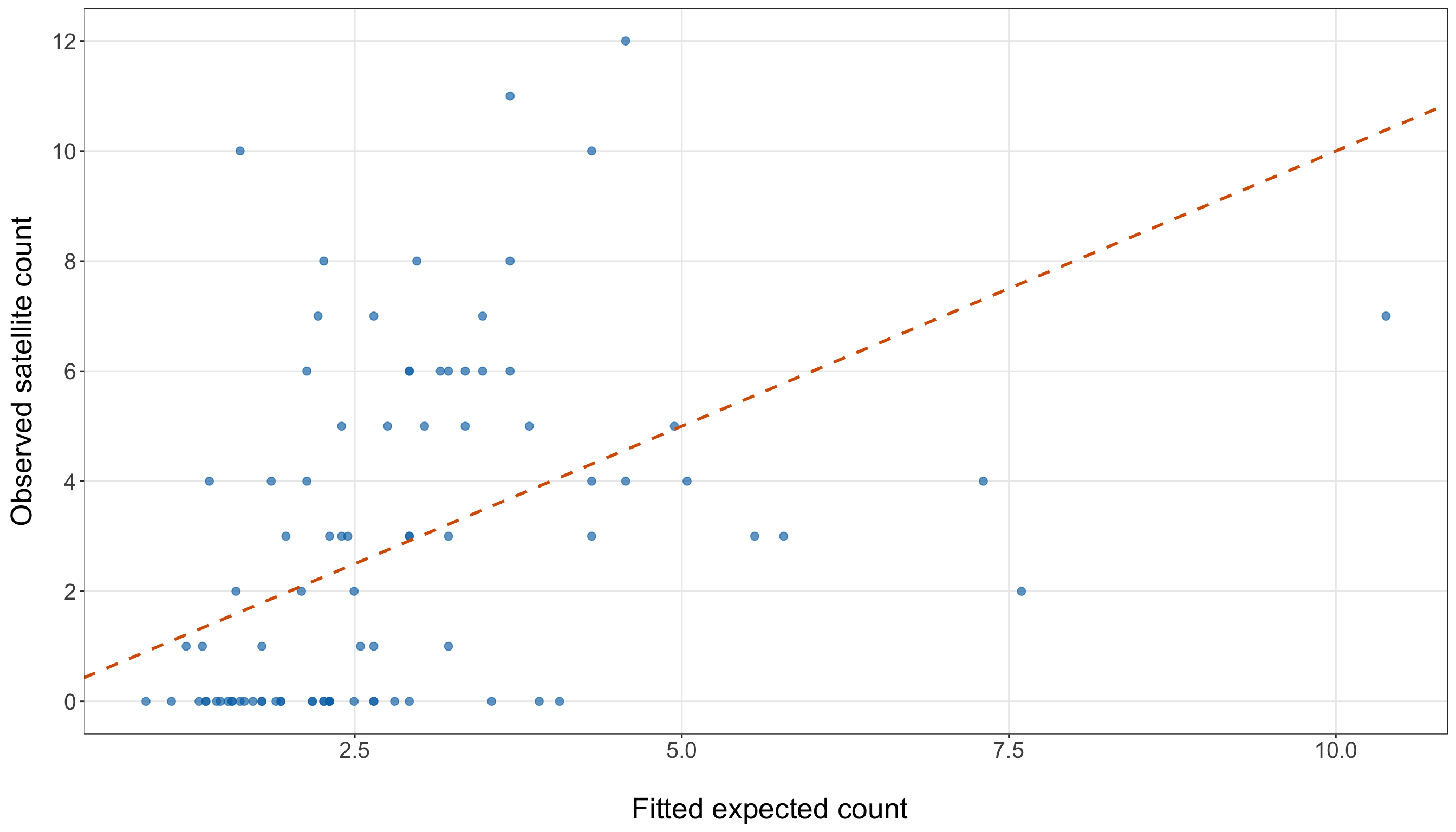
observed_fitted_figure, observed_fitted_axis = plt.subplots(
    figsize=(14, 8)
)

observed_fitted_axis.scatter(
    simple_poisson_gof_data["fitted_expected_count"],
    simple_poisson_gof_data["satellites"],
    alpha=0.65,
    s=35,
    color="#0072B2"
)

line_max = max(
    simple_poisson_gof_data["fitted_expected_count"].max(),
    simple_poisson_gof_data["satellites"].max()
)

observed_fitted_axis.plot(
    [0, line_max],
    [0, line_max],
    linestyle="--",
    linewidth=1,
    color="#D55E00"
)

observed_fitted_axis.set_xlabel(
    "\n Fitted expected count",
    fontsize=20
)

observed_fitted_axis.set_ylabel(
    "Observed satellite count",
    fontsize=20,
    labelpad=12
)

observed_fitted_axis.tick_params(axis="both", labelsize=15.5)
observed_fitted_axis.set_yticks(range(0, 13, 2))

observed_fitted_axis.grid(
    True,
    which="major",
    axis="both",
    alpha=0.3
)

observed_fitted_axis.grid(False, which="minor")

observed_fitted_figure.tight_layout()
plt.show()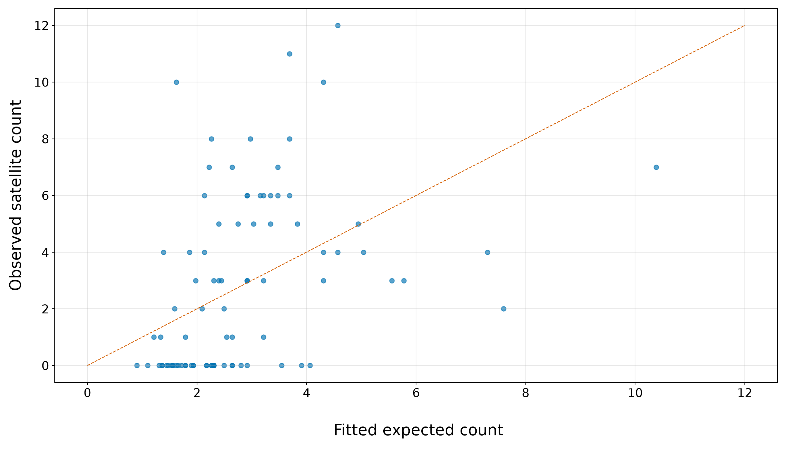
In Figure 10.12 or Figure 10.13, the simple width-only model shows clear signs of strain. For fitted expected counts between roughly \(1.5\) and \(4\), there are many observed zeros sitting well below the dashed line, which is consistent with Table 10.30 showing that the model understates the number of zero satellite counts. At the same time, several observations in this same fitted-count range have much larger observed counts, including values around \(6\), \(8\), \(10\), and higher. This produces a large vertical spread among crabs with similar fitted expected counts.
The horizontal bands in the plot are expected because the observed response is a count. The fitted expected count on the \(x\)-axis is allowed to be fractional, but the observed satellite count on the \(y\)-axis can only take values such as \(0\), \(1\), \(2\), \(3\), and so on. What is concerning is not the banding itself, but the amount of vertical spread around similar fitted expected counts. This pattern suggests that the simple width-only Classical Poisson model is not capturing all the structure in the training data and may be too restrictive in its variance assumption.
10.8.2 Mean-Variance Structure and Equidispersion
The defining mean-variance assumption of Classical Poisson regression is equidispersion:
\[ \mu_i = \mathbb{E}(Y_i \mid \mathbf{x}_i) = \operatorname{Var}(Y_i \mid \mathbf{x}_i). \]
This is a conditional statement. It does not say that the raw sample variance must be exactly equal to the raw sample mean. Instead, it says that after accounting for the regressors included in the model, the remaining conditional variability should be compatible with the fitted Poisson mean-variance structure.
Definition of overdispersion
A count response variable shows overdispersion relative to a Classical Poisson regression model when its conditional variance is larger than the conditional mean allowed by the model. In practice, after accounting for \(k\) regressors, the observed counts vary more than the fitted Poisson model would predict.
Overdispersion is critical because Classical Poisson regression links the conditional mean and conditional variance through the same quantity,
\[ \mu_i = \mathbb{E}(Y_i \mid x_{i,1}, x_{i,2}, \ldots, x_{i,k}) = \operatorname{Var}(Y_i \mid x_{i,1}, x_{i,2}, \ldots, x_{i,k}). \]
If the data are more variable than this structure allows, coefficient estimates may still describe the fitted mean pattern, but standard errors, hypothesis tests, confidence intervals, and prediction uncertainty can become misleading unless the issue is addressed.
A common diagnostic statistic for overdispersion is the Pearson Chi-squared statistic,
\[ X_P^2 = \sum_{i=1}^n \frac{(y_i - \hat{\mu}_i)^2}{\hat{\mu}_i}. \tag{10.14}\]
If the Classical Poisson model is adequate, \(X_P^2\) should be roughly comparable to the residual degrees of freedom,
\[ \nu = n - (k + 1), \]
where \(k + 1\) is the number of estimated regression coefficients, including the intercept. This motivates the Pearson dispersion estimate
\[ \hat{\phi}_P = \frac{X_P^2}{\nu}. \tag{10.15}\]
Values of \(\hat{\phi}_P\) close to \(1\) are consistent with the Classical Poisson mean-variance structure. Values much larger than \(1\) suggest overdispersion.
Then, we can express this as a formal one-sided hypothesis test:
\[ H_0\text{: } \phi = 1 \qquad\text{versus}\qquad H_1\text{: } \phi > 1. \]
Under the null hypothesis and regularity conditions, the Pearson statistic is approximately
\[ X_P^2 \mathrel{\dot{\sim}} \chi^2_{\nu}. \]
Heads-up on regularity conditions for this test!
The phrase “regularity conditions” means that the Chi-squared approximation used in this test relies on some practical assumptions about the fitted model and the data. In this setting, the most important ones are that the observations are independent conditional on the regressors, the fitted expected counts \(\hat{\mu}_i\) are not too close to zero for too many observations, the sample size is large enough for the approximation to be reasonable, and the model is not affected by extreme leverage or a few observations dominating the fit.
These conditions are critical because the reference distribution
\[ X_P^2 \mathrel{\dot{\sim}} \chi^2_{\nu}. \]
is an approximation, not an exact finite-sample result. With small samples, sparse fitted counts, strong dependence among observations, or influential observations, the \(p\)-value from the Pearson Chi-squared test should be treated as a diagnostic signal rather than a definitive yes-or-no decision.
In this chapter, we use the test as one piece of the goodness-of-fit assessment. We will combine it with observed-versus-fitted comparisons, residual deviance, zero-count checks, and the practical modelling goal.
Thus, the overdispersion test \(p\)-value is
\[ p\text{-value} = \Pr \left( \chi^2_{\nu} \geq X_P^2 \right). \]
A small \(p\)-value gives evidence against equidispersion in the direction of overdispersion.
The code below computes each piece of the overdispersion test directly from the fitted simple Poisson regression model. In R, residuals(simple_poisson_width_model, type = "pearson") extracts the Pearson residuals as in Equation 10.13. Squaring these residuals and adding them gives the Pearson Chi-squared statistic from Equation 10.14. Then, the function df.residual(simple_poisson_width_model) extracts the residual degrees of freedom, \(\nu = n - (k + 1)\). We then compute the Pearson dispersion estimate as pearson_chi_squared / pearson_df. Finally, pchisq(pearson_chi_squared, df = pearson_df, lower.tail = FALSE) computes the upper-tail probability
\[ \Pr(\chi^2_{\nu} \geq X_P^2), \]
which is the one-sided overdispersion test \(p\)-value.
The Python code follows the same steps. The fitted {statsmodels} object stores the Pearson residuals in simple_poisson_width_model.resid_pearson and the residual degrees of freedom in simple_poisson_width_model.df_resid. The expression np.sum(simple_poisson_width_model.resid_pearson ** 2) computes \(X_P^2\), and stats.chi2.sf(pearson_chi_squared, pearson_df) computes the same upper-tail Chi-squared probability. The abbreviation sf stands for survival function, which means
\[ 1 - F_{\chi^2_{\nu}}(X_P^2) = \Pr(\chi^2_{\nu} \geq X_P^2). \]
Using the survival function is often numerically more stable than computing 1 - stats.chi2.cdf(...) directly.
Heads-up on the survival function!
In the Python code, stats.chi2.sf(...) uses the survival function of the Chi-squared distribution. Here, the word “survival” does not mean that we are doing survival analysis.
For a random variable \(Z\) with cumulative distribution function \(F_Z(z)\), the survival function is
\[ S_Z(z) = \Pr(Z \geq z) = 1 - F_Z(z). \]
In the overdispersion test, we use the survival function only to compute an upper-tail probability:
\[ \Pr(\chi^2_{\nu} \geq X_P^2). \]
This is a probability calculation for a Chi-squared test statistic, not a time-to-event analysis. Survival analysis is a separate modelling area concerned with outcomes such as event times, censoring, hazard functions, and survival curves. We discuss those ideas in Chapter 6 and Chapter 7.
pearson_chi_squared <- sum(
  residuals(
    simple_poisson_width_model,
    type = "pearson"
  )^2
)

pearson_df <- df.residual(simple_poisson_width_model)

pearson_dispersion <- pearson_chi_squared / pearson_df

pearson_overdispersion_p_value <- pchisq(
  pearson_chi_squared,
  df = pearson_df,
  lower.tail = FALSE
)

overdispersion_summary <- tibble::tibble(
  `Pearson Chi-squared statistic` = pearson_chi_squared,
  `Residual degrees of freedom` = pearson_df,
  `Pearson dispersion estimate` = pearson_dispersion,
  `Overdispersion test p-value` = pearson_overdispersion_p_value
) |>
  mutate(
    `Pearson Chi-squared statistic` = formatC(
      `Pearson Chi-squared statistic`,
      format = "f",
      digits = 3
    ),
    `Residual degrees of freedom` = formatC(
      `Residual degrees of freedom`,
      format = "f",
      digits = 0
    ),
    `Pearson dispersion estimate` = formatC(
      `Pearson dispersion estimate`,
      format = "f",
      digits = 3
    ),
    `Overdispersion test p-value` = formatC(
      `Overdispersion test p-value`,
      format = "e",
      digits = 2
    )
  ) |>
  pivot_longer(
    cols = everything(),
    names_to = "Quantity",
    values_to = "Value"
  )

overdispersion_summary |>
  kable(
    align = c("c", "c")
)| Quantity | Value |
|---|---|
| Pearson Chi-squared statistic | 252.700 |
| Residual degrees of freedom | 84 |
| Pearson dispersion estimate | 3.008 |
| Overdispersion test p-value | 8.61e-19 |
from scipy import stats

pearson_chi_squared = np.sum(
    simple_poisson_width_model.resid_pearson ** 2
)

pearson_df = simple_poisson_width_model.df_resid

pearson_dispersion = pearson_chi_squared / pearson_df

pearson_overdispersion_p_value = stats.chi2.sf(
    pearson_chi_squared,
    pearson_df
)

overdispersion_summary = pd.DataFrame(
    {
        "Quantity": [
            "Pearson Chi-squared statistic",
            "Residual degrees of freedom",
            "Pearson dispersion estimate",
            "Overdispersion test p-value",
        ],
        "Value": [
            f"{pearson_chi_squared:.3f}",
            f"{pearson_df:.0f}",
            f"{pearson_dispersion:.3f}",
            f"{pearson_overdispersion_p_value:.2e}",
        ],
    }
)

classical_poisson_overdispersion_test_py_html = (
    overdispersion_summary.to_html(
        index=False,
        border=0,
    )
)| Quantity | Value |
|---|---|
| Pearson Chi-squared statistic | 252.700 |
| Residual degrees of freedom | 84 |
| Pearson dispersion estimate | 3.008 |
| Overdispersion test p-value | 8.61e-19 |
For this simple width-only model, the Pearson dispersion estimate is 3.008. Since this value is much larger than \(1\), the training data show evidence of overdispersion relative to the simple Classical Poisson model. The \(p\)-value from the one-sided Chi-squared test is 8.61e-19, which provides formal evidence against the equidispersion assumption. Note that this result is necessary for inference. The coefficient estimates can still describe the fitted mean pattern, but the model-based standard errors from the Classical Poisson model rely on equidispersion. If overdispersion is present, those standard errors can be underestimated, making Wald statistics too large, confidence intervals too narrow, and Type I errors more probable.
10.8.3 Excess Zero Counts
In Section 10.5.1, the EDA also showed many zero satellite counts. We now check whether the fitted simple Classical Poisson model expects a similar number of zeros in the training data. Hence, this diagnostic focuses on the number of observed zero counts,
\[ z_{\operatorname{obs}} = \sum_{i=1}^n \mathbb{1}(y_i = 0), \]
where \(\mathbb{1}(y_i = 0)\) is an indicator that equals \(1\) when the \(i\)th observed satellite count is zero and equals \(0\) otherwise.

Under the fitted Classical Poisson model, the probability that the \(i\)th female crab has zero satellite males is
\[ \Pr(Y_i = 0 \mid \mathbf{x}_i; \hat{\boldsymbol{\beta}}_{\operatorname{MLE,obs}}) = \exp(-\hat{\mu}_i). \]
Now, let
\[ \hat{\pi}_{0,i} = \exp(-\hat{\mu}_i) \]
denote this fitted zero probability for observation \(i\). Then, the fitted expected number of zeros in the training data is
\[ \widehat{\mathbb{E}}(Z) = \sum_{i=1}^n \hat{\pi}_{0,i}. \]
The question is whether the observed number of zeros is unusually large compared with what the fitted Classical Poisson model expects. We can frame this as a one-sided diagnostic test:
\[ \begin{gather} H_0\text{: } \text{the fitted Classical Poisson model adequately describes} \\ \text{the frequency of zero counts}, \\ \text{versus} \\ H_1\text{: } \text{there are more zero counts than the} \\ \text{fitted Classical Poisson model expects}. \end{gather} \]
Under \(H_0\), the zero-count indicators \(\mathbb{1}(Y_i = 0)\) are treated as independent Bernoulli random variables with fitted probabilities \(\hat{\pi}_{0,i}\). Because these probabilities can differ across observations, the total number of zeros is a sum of Bernoulli variables with unequal probabilities. Its fitted mean is
\[ \widehat{\mathbb{E}}(Z) = \sum_{i=1}^n \hat{\pi}_{0,i}, \]
and its fitted variance is
\[ \widehat{\operatorname{Var}}(Z) = \sum_{i=1}^n \hat{\pi}_{0,i} (1 - \hat{\pi}_{0,i}). \]
This gives the approximate \(z\)-statistic
\[ z_{\operatorname{zero}} = \frac{ z_{\operatorname{obs}} - \widehat{\mathbb{E}}(Z) }{ \sqrt{ \widehat{\operatorname{Var}}(Z) } }. \tag{10.16}\]
Large positive values of \(z_{\operatorname{zero}}\) indicate that the training data contain more zero counts than the fitted Poisson model expects. The corresponding one-sided \(p\)-value is
\[ \begin{gather} Z_{\operatorname{zero}} \sim \operatorname{Normal}\left(0,1\right) \\ p\text{-value} = \Pr \left( Z_{\operatorname{zero}} \geq z_{\operatorname{zero}} \right), \end{gather} \]
where \(\operatorname{Normal}(0,1)\) denotes a standard Normal random variable.
Heads-up on what this zero-count test is checking!
This diagnostic is not testing whether the response variable can take the value zero. A Poisson model always allows zero counts. Instead, it asks whether the number of zeros observed in the training data is unusually large compared with the number of zeros expected under the fitted Classical Poisson model.
The fitted model can assign a different zero probability to each female crab because each crab has its own fitted expected count \(\hat{\mu}_i\). For the \(i\)th crab, that fitted zero probability is
\[ \hat{\pi}_{0i} = \exp(-\hat{\mu}_i). \]
The fitted expected number of zeros is obtained by adding these fitted zero probabilities across the training observations. If the observed zero count is much larger than this fitted expectation, then the model may be missing a feature of the data-generating process. This can happen, for example, when some female crabs have zero satellite males for reasons not captured by width alone.
This check is a diagnostic, not a final model-selection rule. A large excess of zeros would motivate considering zero-inflated count models (see Chapter 12), but it should be interpreted alongside the overdispersion check, residual deviance, residual plots, and the scientific context.
The following table computes the observed zero count, the fitted expected zero count, the approximate \(z\)-statistic, and the one-sided \(p\)-value.
observed_zero_count <- sum(
  simple_poisson_gof_data$satellites == 0
)

expected_zero_count <- sum(
  simple_poisson_gof_data$fitted_zero_probability
)

zero_count_variance <- sum(
  simple_poisson_gof_data$fitted_zero_probability *
    (1 - simple_poisson_gof_data$fitted_zero_probability)
)

zero_count_z <- (
  observed_zero_count - expected_zero_count
) / sqrt(zero_count_variance)

zero_count_p_value <- pnorm(
  zero_count_z,
  lower.tail = FALSE
)

zero_count_summary <- tibble::tibble(
  `Observed zero count` = observed_zero_count,
  `Fitted expected zero count` = expected_zero_count,
  `Observed minus fitted zeros` = observed_zero_count - expected_zero_count,
  `Approximate z-statistic` = zero_count_z,
  `One-sided p-value` = zero_count_p_value
) |>
  mutate(
    `Observed zero count` = formatC(
      `Observed zero count`,
      format = "f",
      digits = 0
    ),
    `Fitted expected zero count` = formatC(
      `Fitted expected zero count`,
      format = "f",
      digits = 2
    ),
    `Observed minus fitted zeros` = formatC(
      `Observed minus fitted zeros`,
      format = "f",
      digits = 2
    ),
    `Approximate z-statistic` = formatC(
      `Approximate z-statistic`,
      format = "f",
      digits = 2
    ),
    `One-sided p-value` = formatC(
      `One-sided p-value`,
      format = "e",
      digits = 2
    )
  ) |>
  pivot_longer(
    cols = everything(),
    names_to = "Quantity",
    values_to = "Value"
  )

zero_count_summary |>
  kable(
    align = c("c", "c")
)| Quantity | Value |
|---|---|
| Observed zero count | 34 |
| Fitted expected zero count | 8.97 |
| Observed minus fitted zeros | 25.03 |
| Approximate z-statistic | 9.21 |
| One-sided p-value | 1.62e-20 |
observed_zero_count = (
    simple_poisson_gof_data["satellites"] == 0
).sum()

expected_zero_count = (
    simple_poisson_gof_data["fitted_zero_probability"].sum()
)

zero_count_variance = (
    simple_poisson_gof_data["fitted_zero_probability"]
    * (1 - simple_poisson_gof_data["fitted_zero_probability"])
).sum()

zero_count_z = (
    observed_zero_count - expected_zero_count
) / np.sqrt(zero_count_variance)

zero_count_p_value = stats.norm.sf(zero_count_z)

zero_count_summary = pd.DataFrame(
    {
        "Quantity": [
            "Observed zero count",
            "Fitted expected zero count",
            "Observed minus fitted zeros",
            "Approximate z-statistic",
            "One-sided p-value",
        ],
        "Value": [
            f"{observed_zero_count:.0f}",
            f"{expected_zero_count:.2f}",
            f"{observed_zero_count - expected_zero_count:.2f}",
            f"{zero_count_z:.2f}",
            f"{zero_count_p_value:.2e}",
        ],
    }
)

classical_poisson_zero_count_check_py_html = (
    zero_count_summary.to_html(
        index=False,
        border=0,
    )
)| Quantity | Value |
|---|---|
| Observed zero count | 34 |
| Fitted expected zero count | 8.97 |
| Observed minus fitted zeros | 25.03 |
| Approximate z-statistic | 9.21 |
| One-sided p-value | 1.62e-20 |
This zero-count check gives strong evidence that the simple width-only Classical Poisson model is not reproducing the zero-count part of the response distribution. In the training data, the observed number of female crabs with zero satellite males is 34, while the fitted model expects only 8.97 zeros. The difference is therefore 25.03 additional zero counts beyond what the fitted model expects. Then, the approximate \(z\)-statistic is 9.21, with a one-sided \(p\)-value of 1.62e-20. This provides strong diagnostic evidence of excess zero counts relative to the simple Classical Poisson model. In practical terms, the model is not only struggling with the overall mean-variance structure; it is also substantially understating how often zero satellite counts occur in the training data.
Furthermore, this zero-count check should still be interpreted as one diagnostic rather than as the only criterion for choosing a model. However, when combined with the earlier overdispersion evidence from Section 10.8.2, it suggests that the simple Classical Poisson model is too restrictive for these data. This situation motivates a closer look at alternatives such as zero-inflated count models.
10.8.4 Residual Deviance
The overdispersion and zero-count checks each focused on a specific feature of the fitted model. Note that the the Pearson Chi-squared test (in Section 10.8.2) focused on whether the observed counts vary more than the Classical Poisson mean-variance structure allows, while the zero-count check (in Section 10.8.3) focused on whether the model expects enough zero satellite counts.

Now, let us dig into residual deviance. This metric gives a more global goodness-of-fit check. Instead of focusing only on variance or zeros, it compares the likelihood of the fitted regression model with the likelihood of an idealized benchmark model that fits the observed responses as closely as possible. That benchmark is called the saturated model. In this chapter, we use residual deviance as another training-data diagnostic. It will help us ask whether the simple width-only Classical Poisson model is close enough to the observed training counts, relative to what would be possible under a perfect-fit benchmark.
Definition of saturated model
A saturated model is a model that fits the observed data perfectly by using enough parameters to reproduce every observed response value exactly. The saturated model is usually not useful as a practical regression model. Instead, it serves as a theoretical benchmark. Residual deviance compares the fitted model we actually use with this perfect-fit benchmark.
Definition of residual deviance
The residual deviance of a fitted GLM measures how far the fitted regression model is from a saturated model, where the saturated model is the idealized benchmark that fits the observed responses perfectly.
The residual deviance is defined as
\[ D = 2 \left[ \ell_{\operatorname{saturated}} - \ell_{\operatorname{fitted}} \right], \tag{10.17}\]
where \(\ell_{\operatorname{saturated}}\) is the log-likelihood of the saturated model, and \(\ell_{\operatorname{fitted}}\) is the log-likelihood of the fitted regression model.
The factor of \(2\) is included so that, under suitable regularity conditions, the residual deviance can often be compared to a Chi-squared reference distribution. In this sense, residual deviance plays a role similar to a discrepancy measure: smaller values indicate that the fitted model is closer to the saturated benchmark, while larger values indicate that the fitted model is much less likely than a model that reproduces the observed responses exactly.
For Poisson regression, Equation 10.17 can be written as
\[ D = 2 \sum_{i=1}^n \left[ y_i \log\left(\frac{y_i}{\hat{\mu}_i}\right) - (y_i - \hat{\mu}_i) \right], \tag{10.18}\]
where \(n\) is the number of observations used to fit the model, \(y_i\) is the observed count for observation \(i\), and \(\hat{\mu}_i\) is the fitted expected count for observation \(i\). When \(y_i = 0\), the term \(y_i \log(y_i / \hat{\mu}_i)\) is defined to be \(0\).
In practical terms, in Equation 10.18, the residual deviance adds up how much the observed counts differ from the fitted expected counts on the likelihood scale. It is not simply a sum of squared residuals, but it serves a similar diagnostic purpose: it helps us assess whether the fitted model is close enough to the observed data to be considered adequate.
If the fitted Classical Poisson model is adequate, then the gap between the fitted model and the saturated model should not be unusually large. In large samples, this gap is often assessed by comparing the residual deviance to a Chi-squared distribution with residual degrees of freedom
\[ \nu = n - (k + 1), \]
where \(n\) is the number of training observations and \(k + 1\) is the number of estimated regression terms (intercept and coefficients). Under this reference approximation,
\[ D \mathrel{\dot{\sim}} \chi^2_{\nu}. \]
This gives the goodness-of-fit hypotheses
\[ \begin{gather} H_0\text{: } \text{the fitted Classical Poisson model is adequate}, \\ \text{versus} \\ H_1\text{: } \text{the fitted Classical Poisson model is not adequate}. \end{gather} \]
The \(p\)-value is
\[ p\text{-value} = \Pr \left( \chi^2_{\nu} \geq D \right). \]
A small \(p\)-value means that the residual deviance is unusually large under the fitted model, which is evidence of lack of fit.
Heads-up on residual deviance as a global diagnostic!
The residual deviance is a global goodness-of-fit diagnostic. It does not tell us by itself whether the problem is overdispersion, excess zeros, a missing regressor, a nonlinear relationship, influential observations, or some combination of these issues. This is why we do not use residual deviance alone to decide what to do next. Instead, we interpret it alongside more targeted diagnostics, such as the Pearson Chi-squared overdispersion test, the zero-count check, and residual plots.

In this example, a small residual deviance \(p\)-value is a signal that the simple width-only Classical Poisson model is not adequate as a full description of the training data. It does not tell us which alternative model is automatically best.
The code below extracts the residual deviance from the simple fitted model and compares it with its residual degrees of freedom:
- In
R,deviance(simple_poisson_width_model)extracts the residual deviance anddf.residual(simple_poisson_width_model)extracts the residual degrees of freedom. The upper-tail \(p\)-value is computed withpchisq(..., lower.tail = FALSE). - The
Pythoncode follows the same logic. The fitted {statsmodels} object stores the residual deviance insimple_poisson_width_model.devianceand the residual degrees of freedom insimple_poisson_width_model.df_resid. The commandstats.chi2.sf(residual_deviance, residual_deviance_df)computes the same upper-tail Chi-squared probability.
# Residual deviance from the fitted Poisson GLM
residual_deviance <- deviance(simple_poisson_width_model)

# Residual degrees of freedom: n minus the number of estimated terms
residual_deviance_df <- df.residual(simple_poisson_width_model)

# Residual deviance divided by residual degrees of freedom
residual_deviance_ratio <- residual_deviance / residual_deviance_df

# Upper-tail p-value under the Chi-squared reference distribution
residual_deviance_p_value <- pchisq(
  residual_deviance,
  df = residual_deviance_df,
  lower.tail = FALSE
)

residual_deviance_summary <- tibble::tibble(
  `Residual deviance` = residual_deviance,
  `Residual degrees of freedom` = residual_deviance_df,
  `Residual deviance / df` = residual_deviance_ratio,
  `Goodness-of-fit p-value` = residual_deviance_p_value
) |>
  mutate(
    `Residual deviance` = formatC(
      `Residual deviance`,
      format = "f",
      digits = 3
    ),
    `Residual degrees of freedom` = formatC(
      `Residual degrees of freedom`,
      format = "f",
      digits = 0
    ),
    `Residual deviance / df` = formatC(
      `Residual deviance / df`,
      format = "f",
      digits = 3
    ),
    `Goodness-of-fit p-value` = formatC(
      `Goodness-of-fit p-value`,
      format = "e",
      digits = 2
    )
  ) |>
  pivot_longer(
    cols = everything(),
    names_to = "Quantity",
    values_to = "Value"
  )

residual_deviance_summary |>
  kable(
    align = c("c", "c")
)| Quantity | Value |
|---|---|
| Residual deviance | 266.581 |
| Residual degrees of freedom | 84 |
| Residual deviance / df | 3.174 |
| Goodness-of-fit p-value | 7.29e-21 |
# Residual deviance from the fitted Poisson GLM
residual_deviance = simple_poisson_width_model.deviance

# Residual degrees of freedom: n minus the number of estimated terms
residual_deviance_df = simple_poisson_width_model.df_resid

# Residual deviance divided by residual degrees of freedom
residual_deviance_ratio = residual_deviance / residual_deviance_df

# Upper-tail p-value under the Chi-squared reference distribution
residual_deviance_p_value = stats.chi2.sf(
    residual_deviance,
    residual_deviance_df
)

residual_deviance_summary = pd.DataFrame(
    {
        "Quantity": [
            "Residual deviance",
            "Residual degrees of freedom",
            "Residual deviance / df",
            "Goodness-of-fit p-value",
        ],
        "Value": [
            f"{residual_deviance:.3f}",
            f"{residual_deviance_df:.0f}",
            f"{residual_deviance_ratio:.3f}",
            f"{residual_deviance_p_value:.2e}",
        ],
    }
)

classical_poisson_residual_deviance_py_html = (
    residual_deviance_summary.to_html(
        index=False,
        border=0,
    )
)| Quantity | Value |
|---|---|
| Residual deviance | 266.581 |
| Residual degrees of freedom | 84 |
| Residual deviance / df | 3.174 |
| Goodness-of-fit p-value | 7.29e-21 |
For this simple model, the residual deviance is 266.581, while the residual degrees of freedom are 84. The ratio 3.174 is much larger than \(1\), and the corresponding goodness-of-fit \(p\)-value is 7.29e-21. This indicates that the simple width-only Classical Poisson model does not reproduce the training data as well as the fitted model assumptions would require. Hence, the result is consistent with the earlier diagnostics:
- The Pearson Chi-squared test suggested overdispersion.
- The zero-count check showed that the model substantially understates the number of zero satellite counts.
Now, the residual deviance check adds a broader likelihood-based signal of lack of fit. Therefore, taken together, these diagnostics suggest that the fitted mean pattern may capture a useful width association, but the simple Classical Poisson model is too restrictive for these training data.
Note that the residual deviance gives a single global statistic. To see where some of the lack of fit may be appearing, we can also inspect Pearson residuals against fitted expected counts. As indicated in Section 10.8.4, Pearson residuals standardize the difference between the observed count and the fitted expected count by the Poisson standard deviation implied by the model:
\[ r_i^{(P)} = \frac{y_i - \hat{\mu}_i}{\sqrt{\hat{\mu}_i}}. \]
pearson_residual_plot <- ggplot(
  simple_poisson_gof_data,
  aes(x = fitted_expected_count, y = pearson_residual)
) +
  geom_hline(
    yintercept = 0,
    linetype = "solid",
    linewidth = 0.8,
    colour = "grey40"
  ) +
  geom_hline(
    yintercept = c(-2, 2),
    linetype = "dashed",
    linewidth = 0.8,
    colour = "#D55E00"
  ) +
  geom_point(
    alpha = 0.65,
    size = 2.3,
    colour = "#0072B2"
  ) +
  theme_bw() +
  theme(
    axis.text = element_text(size = 15.5),
    axis.title.x = element_text(size = 20),
    axis.title.y = element_text(
      size = 20,
      vjust = 0.5,
      margin = margin(r = 12)
    ),
    panel.grid.minor = element_blank()
  ) +
  labs(
    x = "\n Fitted expected count",
    y = "Pearson residual"
  )

pearson_residual_plot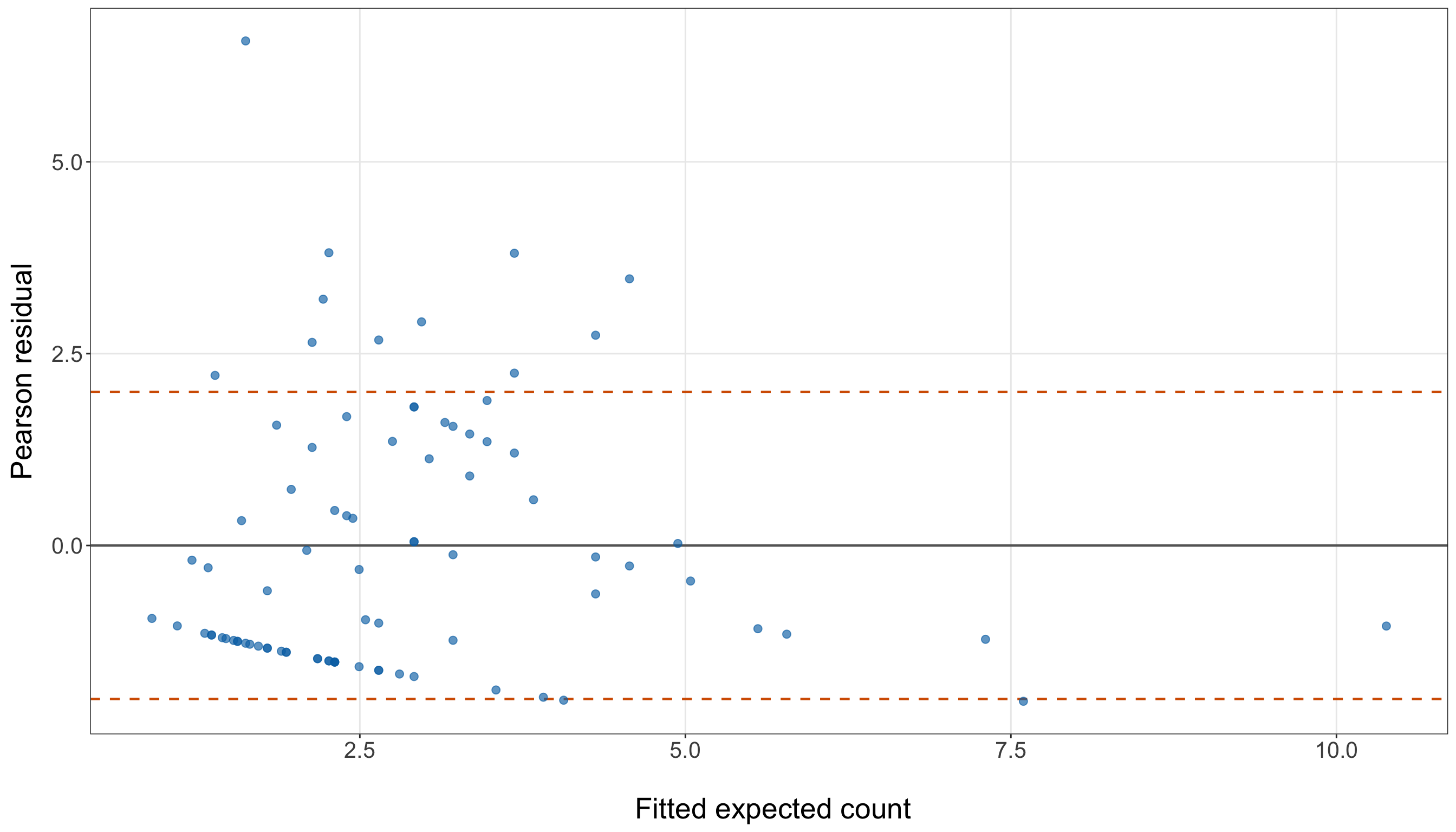
pearson_residual_figure, pearson_residual_axis = plt.subplots(
    figsize=(14, 8)
)

pearson_residual_axis.axhline(
    0,
    linestyle="-",
    linewidth=0.8,
    color="grey"
)

pearson_residual_axis.axhline(
    2,
    linestyle="--",
    linewidth=0.8,
    color="#D55E00"
)

pearson_residual_axis.axhline(
    -2,
    linestyle="--",
    linewidth=0.8,
    color="#D55E00"
)

pearson_residual_axis.scatter(
    simple_poisson_gof_data["fitted_expected_count"],
    simple_poisson_gof_data["pearson_residual"],
    alpha=0.65,
    s=35,
    color="#0072B2"
)

pearson_residual_axis.set_xlabel(
    "\n Fitted expected count",
    fontsize=20
)

pearson_residual_axis.set_ylabel(
    "Pearson residual",
    fontsize=20,
    labelpad=12
)

pearson_residual_axis.tick_params(axis="both", labelsize=15.5)

pearson_residual_axis.grid(
    True,
    which="major",
    axis="both",
    alpha=0.3
)

pearson_residual_axis.grid(False, which="minor")

pearson_residual_figure.tight_layout()
plt.show()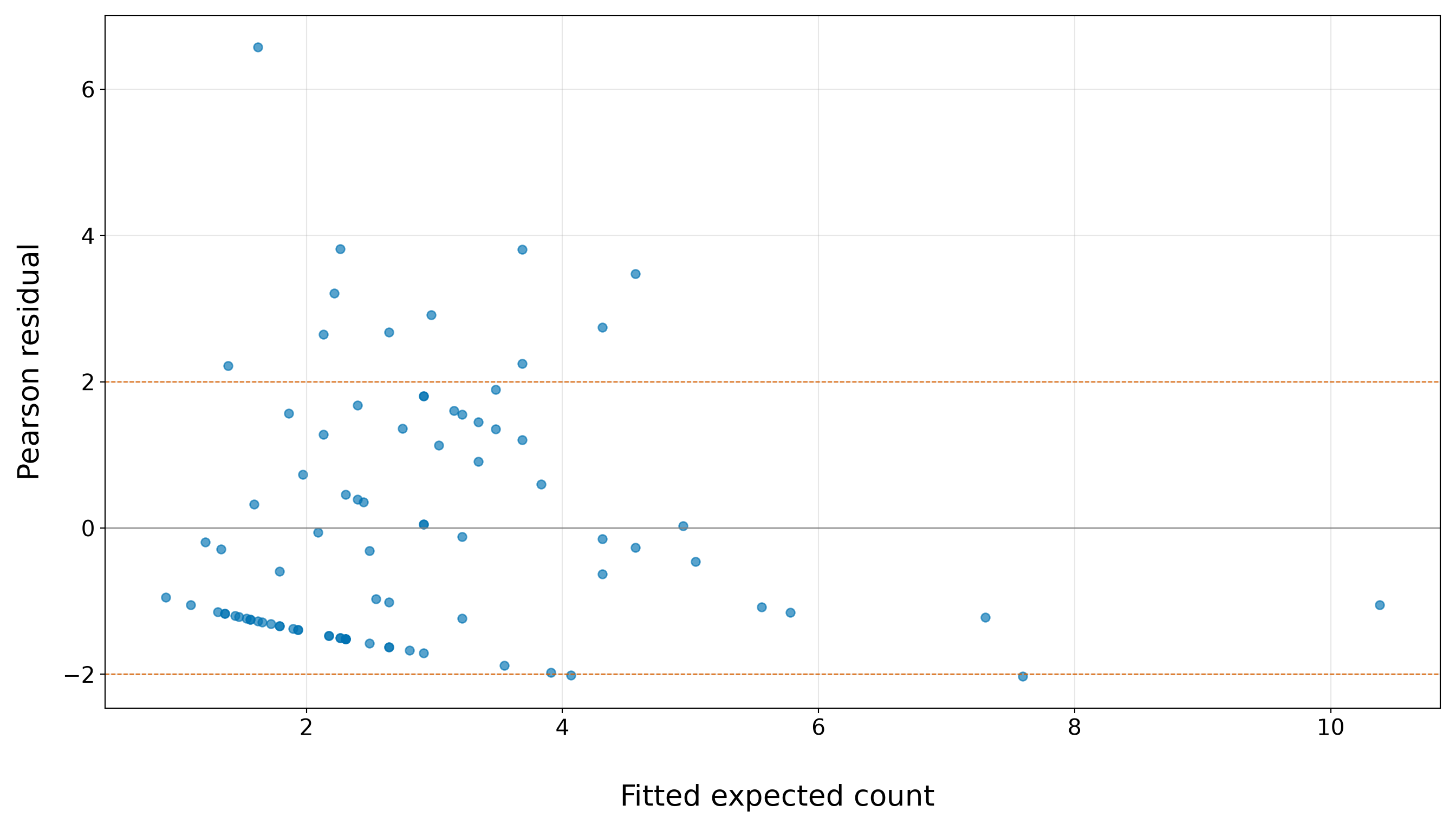
In Figure 10.14 (or Figure 10.15) the solid horizontal line at \(0\) represents a perfect residual balance: the observed count equals the fitted expected count after standardizing by the fitted Poisson standard deviation. The two dashed horizontal lines are visual reference bands at approximately \(-2\) and \(2\). They are not formal decision cutoffs, but they help us identify observations whose Pearson residuals are large in magnitude. Under a reasonably adequate Classical Poisson variance structure, we would expect most Pearson residuals to fall inside these bands, without a strong pattern across fitted expected counts.
However, in the above plot, the residual pattern is not reassuring. Several observations have Pearson residuals above \(2\), including one very large positive residual above \(6\). These are female crabs whose observed satellite counts are much larger than the fitted Poisson model expects, after accounting for the fitted Poisson standard deviation. At the same time, many observations with fitted expected counts between roughly \(1.5\) and \(4\) have negative Pearson residuals, forming a visible lower band. These are mostly zero or small observed counts sitting below their fitted expected counts.
All these patterns are critical. The plot shows both unusually large positive residuals and many negative residuals associated with zero counts. In other words, the simple width-only model is not just missing a few isolated observations; it is struggling to represent the spread and shape of the count distribution. This visual pattern supports the same conclusion as the Pearson Chi-squared test, the excess-zero check, and the residual deviance check: the Classical Poisson mean-variance structure is too restrictive for these training data.
10.8.5 Practical Model Adequacy
Now, we combine the diagnostic evidence. The goal is not to declare the model perfect or useless based on a single number. Instead, we ask whether the simple width-only Classical Poisson model is adequate enough for the next stage of the workflow.
| Diagnostic | What we checked | What the training data suggest | Practical implication |
|---|---|---|---|
| Observed versus fitted counts | Whether fitted expected counts track observed counts across the training data. | The model captures a broad increase in expected counts with width, but individual counts show large variability around the fitted expectations (see Figure 10.12 or Figure 10.13). | Width is useful, but the simple model is not a complete description of the response. |
| Pearson overdispersion test | Whether the conditional variance is compatible with the Classical Poisson mean-variance structure. | The Pearson dispersion estimate is much larger than \(1\), and the overdispersion \(p\)-value is very small. | The model-based standard errors from the simple Poisson model are likely too small. |
| Zero-count check | Whether the fitted model expects a similar number of zeros as observed. | If the observed zero count is larger than the fitted expected zero count, the model is not reproducing the zero-count part of the distribution. | Excess zeros may motivate a zero-inflated model in a later chapter. |
| Residual deviance | Whether the fitted model is close enough to a saturated benchmark. | The residual deviance is much larger than its degrees of freedom, with a very small goodness-of-fit \(p\)-value. | There is formal evidence of lack of fit for the simple Classical Poisson model. |
| Pearson residual plot | Whether residuals show unusually large discrepancies relative to the fitted Poisson variance. | Large residuals and broad residual spread support the overdispersion conclusion (see Figure 10.14 or Figure 10.15). | The simple model is too restrictive as a final inferential model. |
The overall diagnostic picture is not favourable for the simple width-only Classical Poisson model. The model is useful as a starting point because it captures an interpretable width-based mean pattern, but it does not adequately reproduce the variability in the training counts. Moreover, the overdispersion and deviance checks both indicate lack of fit, and the zero-count check may indicate that the model is also underestimating the number of zeros.
In our full data science workflow, this is the point where we would consider returning to the data modelling stage. Several alternatives are possible:
- Add regressors such as weight, colour, and spine condition if the current systematic component is too simple.
- Add nonlinear terms or interactions if the relationship between regressors and expected counts is not adequately captured by the current structure.
- Use a Negative Binomial regression model when the main issue is overdispersion (see Chapter 11).
- Use a Zero-Inflated Poisson regression model when the main issue is an excess of zeros (see Chapter 12).
- Use a Generalized Poisson regression model when the count response departs from the Classical Poisson mean-variance structure in a more flexible way (see Chapter 13).
For learning purposes, we will continue with Classical Poisson regression in this chapter. This does not mean that the simple width-only model has passed all goodness-of-fit checks. Rather, it lets us show how Classical Poisson regression is fitted, checked, extended, interpreted, and used in practice. The diagnostic concerns raised here will remain important context when we extend the model with additional regressors and when later chapters introduce count models designed for overdispersed or zero-heavy responses.
10.9 Extending the Model with Additional Regressors
In Table 10.38, the goodness-of-fit checks for the simple width-only model showed clear diagnostic problems. The model captured a useful width-based mean pattern, but it did not adequately reproduce the variability, zero-count frequency, or global likelihood structure of the training counts. In the data science workflow, this is a natural point to return to the data modelling and estimation stages rather than moving directly to final conclusions.

We now extend the Classical Poisson regression model by adding the remaining explanatory variables available in the horseshoe crab dataset. Hence, this means retaking the same modelling cycle:
- Define the model notation carefully.
- Encode the categorical regressors using dummy variables.
- Estimate the extended model on the training data.
- Revisit goodness of fit on the training data.
- Interpret the fitted mean structure, and prepare predictions for held-out testing observations.
We still fit and diagnose the model using the training data. Then, the testing data remain reserved for the later results section, where we will evaluate final predictive performance and produce final inferential outputs according to the chapter workflow.
10.9.1 Adding Phenotypic Regressors
Recall the notation introduced in Table 10.7. The response is \(Y_i\), the observed number of satellite males for the \(i\)th female crab. The continuous regressors are:
- \(x_{i,1}\): female crab carapace width in centimetres;
- \(x_{i,2}\): female crab weight in kilograms.
The remaining regressors are categorical. As in the data modelling example from Chapter 1, we represent categorical variables by creating binary dummy variables (see Table 1.8). If a categorical variable has \(u\) levels, we use \(u - 1\) dummy variables and leave one level as the baseline or reference category. The baseline category is represented by all zeros for that categorical variable.
Before defining the dummy variables, we first verify the order of the categorical levels. This is necessary because the baseline category is the level represented by all dummy variables equal to zero. For this model, Light is the baseline category for color and Both good is the baseline category for spine since these two categories appear on the left-hand side of the coding output.
color_order = [
    "Light",
    "Medium light",
    "Medium dark",
    "Dark",
]

spine_order = [
    "Both good",
    "One worn or broken",
    "Both worn or broken",
]

training_data["color"] = pd.Categorical(
    training_data["color"],
    categories=color_order
)

training_data["spine"] = pd.Categorical(
    training_data["spine"],
    categories=spine_order
)

training_data["color"].cat.categories
Index(['Light', 'Medium light', 'Medium dark', 'Dark'], dtype='str')training_data["spine"].cat.categoriesIndex(['Both good', 'One worn or broken', 'Both worn or broken'], dtype='str')For color, we use Light as the baseline category. Since color has four levels, we need three dummy variables:
\[ x_{i,3} = \begin{cases} 1, & \text{if the } i\text{th female crab has colour Medium light}, \\ 0, & \text{otherwise}; \end{cases} \]
\[ x_{i,4} = \begin{cases} 1, & \text{if the } i\text{th female crab has colour Medium dark}, \\ 0, & \text{otherwise}; \end{cases} \]
and
\[ x_{i,5} = \begin{cases} 1, & \text{if the } i\text{th female crab has colour Dark}, \\ 0, & \text{otherwise}. \end{cases} \]
Thus, a female crab in the Light colour category has
\[ x_{i,3}=x_{i,4}=x_{i,5}=0. \]
For spine, we use Both good as the baseline category. Since spine has three levels, we need two dummy variables:
\[ x_{i,6} = \begin{cases} 1, & \text{if the } i\text{th female crab has one worn or broken spine}, \\ 0, & \text{otherwise}; \end{cases} \]
and
\[ x_{i,7} = \begin{cases} 1, & \text{if the } i\text{th female crab has both spines worn or broken}, \\ 0, & \text{otherwise}. \end{cases} \]
Thus, a female crab in the Both good spine category has
\[ x_{i,6}=x_{i,7}=0. \]
The full dummy-variable arrangement is summarized in Table 10.39.
| Original variable | Baseline category | Dummy variable | Dummy equals \(1\) when… | Dummy equals \(0\) when… |
|---|---|---|---|---|
color |
Light |
\(x_{i,3}\) |
color is Medium light
|
otherwise |
color |
Light |
\(x_{i,4}\) |
color is Medium dark
|
otherwise |
color |
Light |
\(x_{i,5}\) |
color is Dark
|
otherwise |
spine |
Both good |
\(x_{i,6}\) |
spine is One worn or broken
|
otherwise |
spine |
Both good |
\(x_{i,7}\) |
spine is Both worn or broken
|
otherwise |
Heads-up on reference categories and dummy variables!
The reference category is not omitted because it is unimportant. It is omitted from the dummy-variable list because its information is carried by the intercept and by the fact that all dummy variables for that categorical regressor equal zero.
For colour, Light is the reference category. For spine condition, Both good is the reference category. Therefore, categorical coefficients in the extended model are interpreted relative to these baseline categories, holding the other regressors fixed.
Using this notation, the extended Classical Poisson regression model is
\[ Y_i \mid x_{i,1}, x_{i,2}, \ldots, x_{i,7} \sim \operatorname{Poisson}(\mu_i), \]
with
\[ \begin{aligned} \log(\mu_i) = &\ \beta_0 + \beta_1 x_{i,1} + \beta_2 x_{i,2} + \beta_3 x_{i,3} + \beta_4 x_{i,4} \\ &+ \beta_5 x_{i,5} + \beta_6 x_{i,6} + \beta_7 x_{i,7}. \end{aligned} \tag{10.19}\]
Equivalently,
\[ \mu_i = \exp \left( \beta_0 + \beta_1 x_{i,1} + \beta_2 x_{i,2} + \cdots + \beta_7 x_{i,7} \right). \tag{10.20}\]
This extended model uses the same Classical Poisson random component and log link as before. What changes is the systematic component: instead of using width alone, we now use width, weight, and dummy variables for colour and spine condition.
Heads-up on adding regressors after a failed goodness-of-fit check!
Adding regressors can improve a model when the original systematic component was too simple. For example, if weight, colour, or spine condition explain differences in satellite counts that width alone did not capture, then the extended model may fit the training data better.
However, adding regressors does not automatically fix overdispersion or excess zeros. Overdispersion and zero inflation are distributional problems, not only mean-structure problems. Therefore, after fitting the extended Classical Poisson model, we must repeat the goodness-of-fit checks rather than assuming that the additional regressors solved the diagnostic issues.
Now, we fit the extended model on the training data:
- In
R, the formulasatellites ~ width_cm + weight_kg + color + spinetellsglm()to create the needed dummy variables for the categorical regressors automatically, using the first factor level as the reference category. - In
Python, via Listing 10.7, we explicitly set the categorical order and reference categories so that the fitted model matches the same dummy-variable setup. Then, we fit the corresponding extended model.
extended_poisson_model <- glm(
  satellites ~ width_cm + weight_kg + color + spine,
  family = poisson(link = "log"),
  data = training_data
)

extended_poisson_summary <- tidy(
  extended_poisson_model
) |>
  mutate(
    exponentiated_estimate = exp(estimate),
    percent_change = 100 * (exponentiated_estimate - 1),
    across(
      where(is.numeric),
      ~ round(.x, 2)
    )
  ) |>
  select(
    term,
    estimate,
    std.error,
    exponentiated_estimate,
    percent_change
  )

extended_poisson_summary |>
  rename(
    `Term` = term,
    `Estimate` = estimate,
    `Standard error` = std.error,
    `Exponentiated estimate` = exponentiated_estimate,
    `Percent change` = percent_change
  ) |>
  kable(
    align = c("c", "c", "c", "c", "c")
)| Term | Estimate | Standard error | Exponentiated estimate | Percent change |
|---|---|---|---|---|
| (Intercept) | -1.65 | 1.26 | 0.19 | -80.77 |
| width_cm | 0.05 | 0.06 | 1.05 | 4.60 |
| weight_kg | 0.58 | 0.21 | 1.79 | 79.42 |
| colorMedium light | -0.35 | 0.23 | 0.71 | -29.45 |
| colorMedium dark | -0.48 | 0.27 | 0.62 | -38.22 |
| colorDark | -0.86 | 0.33 | 0.42 | -57.54 |
| spineOne worn or broken | 0.00 | 0.35 | 1.00 | 0.06 |
| spineBoth worn or broken | 0.51 | 0.19 | 1.66 | 66.43 |
extended_poisson_training_data = training_data.copy()

extended_poisson_model = smf.glm(
    formula=(
        "satellites ~ width_cm + weight_kg "
        "+ C(color, Treatment(reference='Light')) "
        "+ C(spine, Treatment(reference='Both good'))"
    ),
    data=extended_poisson_training_data,
    family=sm.families.Poisson()
).fit()

extended_poisson_summary = pd.DataFrame(
    {
        "Term": extended_poisson_model.params.index,
        "Estimate": extended_poisson_model.params.values,
        "Standard error": extended_poisson_model.bse.values,
        "Exponentiated estimate": np.exp(
            extended_poisson_model.params.values
        ),
    }
)

extended_poisson_summary["Percent change"] = (
    100 * (extended_poisson_summary["Exponentiated estimate"] - 1)
)

extended_poisson_summary = extended_poisson_summary.round(2)

classical_poisson_extended_model_fit_py_html = (
    extended_poisson_summary.to_html(
        index=False,
        border=0,
    )
)| Term | Estimate | Standard error | Exponentiated estimate | Percent change |
|---|---|---|---|---|
| Intercept | -1.65 | 1.26 | 0.19 | -80.77 |
| C(color, Treatment(reference=‘Light’))[T.Medium light] | -0.35 | 0.23 | 0.71 | -29.45 |
| C(color, Treatment(reference=‘Light’))[T.Medium dark] | -0.48 | 0.27 | 0.62 | -38.22 |
| C(color, Treatment(reference=‘Light’))[T.Dark] | -0.86 | 0.33 | 0.42 | -57.54 |
| C(spine, Treatment(reference=‘Both good’))[T.One worn or broken] | 0.00 | 0.35 | 1.00 | 0.06 |
| C(spine, Treatment(reference=‘Both good’))[T.Both worn or broken] | 0.51 | 0.19 | 1.66 | 66.43 |
| width_cm | 0.05 | 0.06 | 1.05 | 4.60 |
| weight_kg | 0.58 | 0.21 | 1.79 | 79.42 |
Table 10.40 reports estimates, model-based standard errors, exponentiated estimates, and percent changes. We intentionally do not conduct Wald tests here. Hypothesis testing and final coefficient-level inferential decisions are saved for the later results section, after the model-building workflow has been completed.
10.9.2 Extended Goodness-of-Fit Checks
Now, before interpreting the coefficients, we repeat the goodness-of-fit checks for the extended model. Since the simple width-only model showed overdispersion, excess zeros, and a large residual deviance, we now ask whether adding weight_kg, color, and spine improved those same diagnostics. We will use the same diagnostic tools developed for the simple model, but we will organize them more efficiently here. The goal is not to rederive the mathematics. Instead, we reuse the same ideas to assess whether the extended Classical Poisson model is more adequate on the training data.

Creating Extended-Model Diagnostic Quantities
The first step is to create the fitted expected counts, Pearson residuals, and fitted zero probabilities for the extended model. These are the same diagnostic quantities used for the simple model in Section 10.8, but now they come from the model with all available regressors.
extended_poisson_gof_data = training_data.copy()

extended_poisson_gof_data["fitted_expected_count"] = (
    extended_poisson_model.fittedvalues
)

extended_poisson_gof_data["pearson_residual"] = (
    (
        extended_poisson_gof_data["satellites"]
        - extended_poisson_gof_data["fitted_expected_count"]
    )
    / np.sqrt(extended_poisson_gof_data["fitted_expected_count"])
)

extended_poisson_gof_data["fitted_zero_probability"] = np.exp(
    -extended_poisson_gof_data["fitted_expected_count"]
)
These quantities let us reuse the same goodness-of-fit logic from the simple model from Section 10.8.1. The fitted expected counts \(\hat{\mu}_i\) summarize the fitted mean structure, the Pearson residuals (see Equation 10.13) compare observed and fitted counts relative to the fitted Poisson standard deviation, and the fitted zero probabilities \(\exp(-\hat{\mu}_i)\) tell us how often the extended model expects zero satellite counts.
Extended Observed versus Fitted Counts
Before revisiting overdispersion, zero counts, and residual deviance, we first compare the observed satellite counts with the fitted expected counts from the extended model. This mirrors the observed-versus-fitted check from Section 10.8.1, but now the fitted expected counts come from the model that includes width, weight, colour, and spine condition. This check is still based on the training data. The goal is not to measure held-out prediction accuracy yet. Instead, we are asking whether the extended model’s fitted expected counts are better aligned with the observed count distribution than the simple width-only model.

We start by grouping observations into quartiles based on their fitted expected counts. Within each group, we compare the mean observed count with the mean fitted expected count and also compare the observed zero proportion with the average fitted probability of zero satellite counts.
extended_fitted_count_calibration <- extended_poisson_gof_data |>
  mutate(
    fitted_count_quartile = ntile(fitted_expected_count, 4),
    fitted_count_quartile = factor(
      fitted_count_quartile,
      levels = 1:4,
      labels = c(
        "Q1: smallest fitted counts",
        "Q2",
        "Q3",
        "Q4: largest fitted counts"
      )
    )
  ) |>
  group_by(fitted_count_quartile) |>
  summarise(
    n = n(),
    mean_observed_count = mean(satellites),
    mean_fitted_expected_count = mean(fitted_expected_count),
    observed_zero_proportion = mean(satellites == 0),
    mean_fitted_zero_probability = mean(fitted_zero_probability),
    .groups = "drop"
  ) |>
  mutate(
    across(
      where(is.numeric),
      ~ round(.x, 3)
    )
  )

extended_fitted_count_calibration |>
  rename(
    `Fitted-count quartile` = fitted_count_quartile,
    `Number of female crabs` = n,
    `Mean observed count` = mean_observed_count,
    `Mean fitted expected count` = mean_fitted_expected_count,
    `Observed zero proportion` = observed_zero_proportion,
    `Average fitted probability of zero satellites` =
      mean_fitted_zero_probability
  ) |>
  kable(
    align = c("c", "c", "c", "c", "c", "c")
)| Fitted-count quartile | Number of female crabs | Mean observed count | Mean fitted expected count | Observed zero proportion | Average fitted probability of zero satellites |
|---|---|---|---|---|---|
| Q1: smallest fitted counts | 22 | 0.773 | 1.207 | 0.773 | 0.307 |
| Q2 | 22 | 1.864 | 2.108 | 0.455 | 0.126 |
| Q3 | 21 | 3.952 | 3.071 | 0.238 | 0.049 |
| Q4: largest fitted counts | 21 | 4.952 | 5.122 | 0.095 | 0.010 |
extended_fitted_count_calibration_data = extended_poisson_gof_data.copy()

extended_fitted_count_calibration_data = (
    extended_fitted_count_calibration_data
    .sort_values(
        "fitted_expected_count",
        kind="mergesort"
    )
    .reset_index(drop=True)
)

number_of_rows = len(extended_fitted_count_calibration_data)
number_of_groups = 4

base_group_size = number_of_rows // number_of_groups
remainder = number_of_rows % number_of_groups

group_sizes = [
    base_group_size + 1 if group_index < remainder else base_group_size
    for group_index in range(number_of_groups)
]

fitted_count_quartile_labels = [
    "Q1: smallest fitted counts",
    "Q2",
    "Q3",
    "Q4: largest fitted counts",
]

extended_fitted_count_calibration_data["fitted_count_quartile"] = np.repeat(
    fitted_count_quartile_labels,
    group_sizes
)

extended_fitted_count_calibration_data["fitted_count_quartile"] = (
    pd.Categorical(
        extended_fitted_count_calibration_data["fitted_count_quartile"],
        categories=fitted_count_quartile_labels,
        ordered=True
    )
)

extended_fitted_count_calibration = (
    extended_fitted_count_calibration_data
    .groupby("fitted_count_quartile", observed=False)
    .agg(
        n=("satellites", "size"),
        mean_observed_count=("satellites", "mean"),
        mean_fitted_expected_count=("fitted_expected_count", "mean"),
        observed_zero_proportion=("satellites", lambda x: (x == 0).mean()),
        mean_fitted_zero_probability=("fitted_zero_probability", "mean"),
    )
    .reset_index()
    .round(3)
)

extended_fitted_count_calibration_display = (
    extended_fitted_count_calibration
    .rename(
        columns={
            "fitted_count_quartile": "Fitted-count quartile",
            "n": "Number of female crabs",
            "mean_observed_count": "Mean observed count",
            "mean_fitted_expected_count": "Mean fitted expected count",
            "observed_zero_proportion": "Observed zero proportion",
            "mean_fitted_zero_probability": (
                "Average fitted probability of zero satellites"
            ),
        }
    )
)

classical_poisson_extended_fitted_count_calibration_py_html = (
    extended_fitted_count_calibration_display.to_html(
        index=False,
        border=0,
    )
)| Fitted-count quartile | Number of female crabs | Mean observed count | Mean fitted expected count | Observed zero proportion | Average fitted probability of zero satellites |
|---|---|---|---|---|---|
| Q1: smallest fitted counts | 22 | 0.773 | 1.207 | 0.773 | 0.307 |
| Q2 | 22 | 1.864 | 2.108 | 0.455 | 0.126 |
| Q3 | 21 | 3.952 | 3.071 | 0.238 | 0.049 |
| Q4: largest fitted counts | 21 | 4.952 | 5.122 | 0.095 | 0.010 |
The grouped comparison in Table 10.42 shows that the extended model captures the broad ordering of the fitted mean structure: both the mean observed count and the mean fitted expected count generally increase from the lowest fitted-count quartile to the highest fitted-count quartile. However, the calibration is still uneven across the groups:
- In Q1, the model overestimates the mean count: the mean observed count is 0.773, while the mean fitted expected count is 1.207.
- In Q2, the model is closer, with a mean observed count of 1.864 and a mean fitted expected count of 2.108.
- In Q3, the model underestimates the mean count more noticeably: the mean observed count is 3.952, while the mean fitted expected count is 3.071.
- In Q4, the model slightly overestimates the mean count, with a mean observed count of 4.952 and a mean fitted expected count of 5.122.
The zero-count columns show a more persistent diagnostic problem. In every fitted-count quartile, the observed zero proportion is larger than the average fitted probability of zero satellites. The discrepancy is especially large in Q1, where the observed zero proportion is 0.773, while the average fitted probability of zero satellites is only 0.307. Even in Q4, where the fitted expected counts are largest, the observed zero proportion is 0.095, while the average fitted probability of zero satellites is only 0.01. Thus, adding weight, colour, and spine condition improves the mean structure, but it does not remove the zero-count mismatch. The extended Classical Poisson model still expects fewer zero satellite counts than we observe across the fitted-count range, which prepares us for the formal zero-count diagnostic below.
We can also inspect the same comparison graphically.
extended_observed_fitted_plot <- ggplot(
  extended_poisson_gof_data,
  aes(x = fitted_expected_count, y = satellites)
) +
  geom_point(
    alpha = 0.65,
    size = 2.3,
    colour = "#0072B2"
  ) +
  geom_abline(
    intercept = 0,
    slope = 1,
    linetype = "dashed",
    linewidth = 1,
    colour = "#D55E00"
  ) +
  theme_bw() +
  theme(
    axis.text = element_text(size = 15.5),
    axis.title.x = element_text(size = 20),
    axis.title.y = element_text(
      size = 20,
      vjust = 0.5,
      margin = margin(r = 12)
    ),
    panel.grid.minor = element_blank()
  ) +
  labs(
    x = "\n Fitted expected count",
    y = "Observed satellite count"
  ) +
  scale_y_continuous(breaks = seq(0, 12, by = 2))

extended_observed_fitted_plot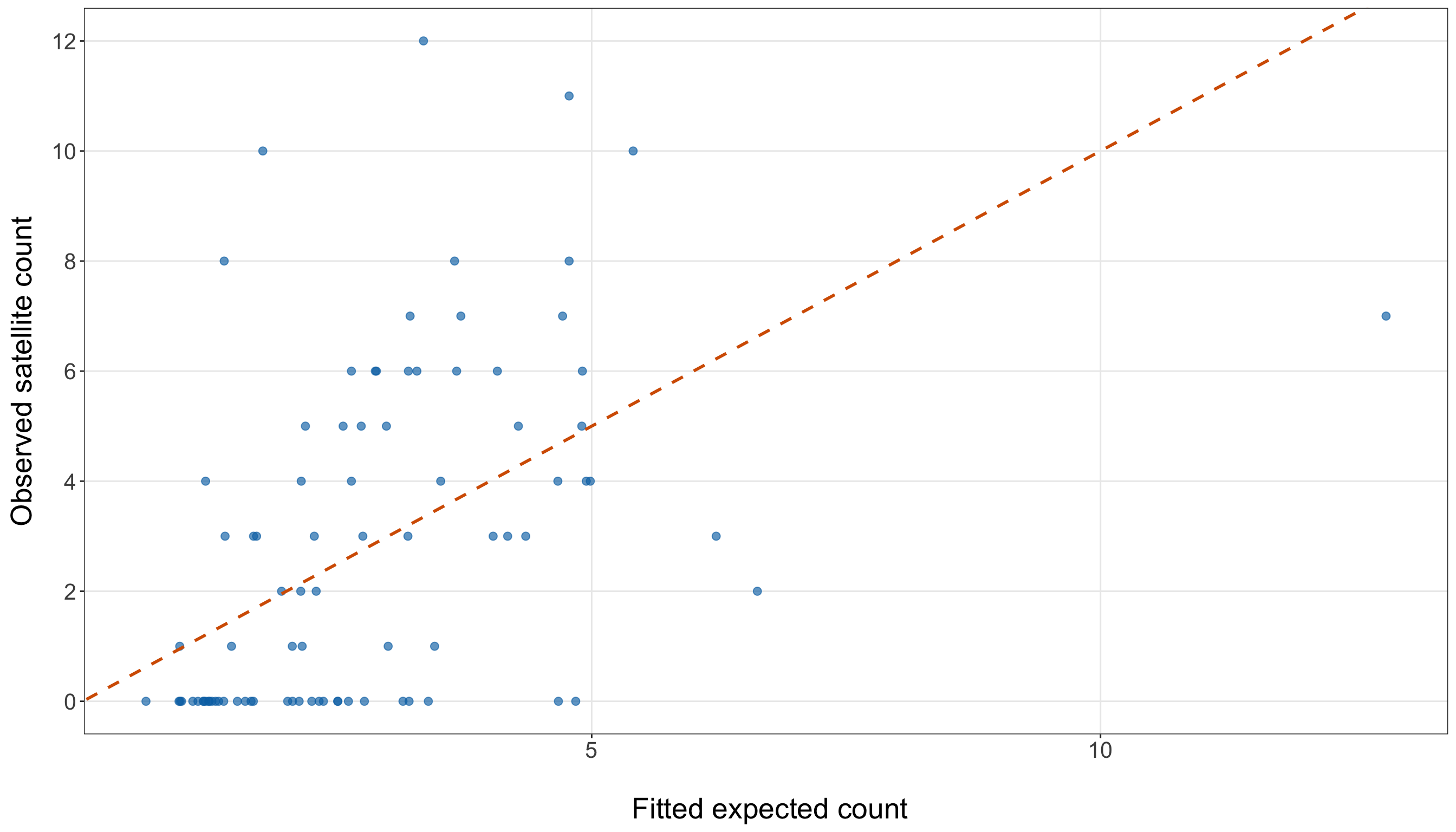
extended_observed_fitted_figure, extended_observed_fitted_axis = (
    plt.subplots(
        figsize=(14, 8)
    )
)

extended_observed_fitted_axis.scatter(
    extended_poisson_gof_data["fitted_expected_count"],
    extended_poisson_gof_data["satellites"],
    alpha=0.65,
    s=35,
    color="#0072B2"
)

extended_line_max = max(
    extended_poisson_gof_data["fitted_expected_count"].max(),
    extended_poisson_gof_data["satellites"].max()
)

extended_observed_fitted_axis.plot(
    [0, extended_line_max],
    [0, extended_line_max],
    linestyle="--",
    linewidth=1,
    color="#D55E00"
)

extended_observed_fitted_axis.set_xlabel(
    "\n Fitted expected count",
    fontsize=20
)

extended_observed_fitted_axis.set_ylabel(
    "Observed satellite count",
    fontsize=20,
    labelpad=12
)

extended_observed_fitted_axis.tick_params(
    axis="both",
    labelsize=15.5
)

extended_observed_fitted_axis.set_yticks(
    range(0, 13, 2)
)

extended_observed_fitted_axis.grid(
    True,
    which="major",
    axis="both",
    alpha=0.3
)

extended_observed_fitted_axis.grid(
    False,
    which="minor"
)

extended_observed_fitted_figure.tight_layout()
plt.show()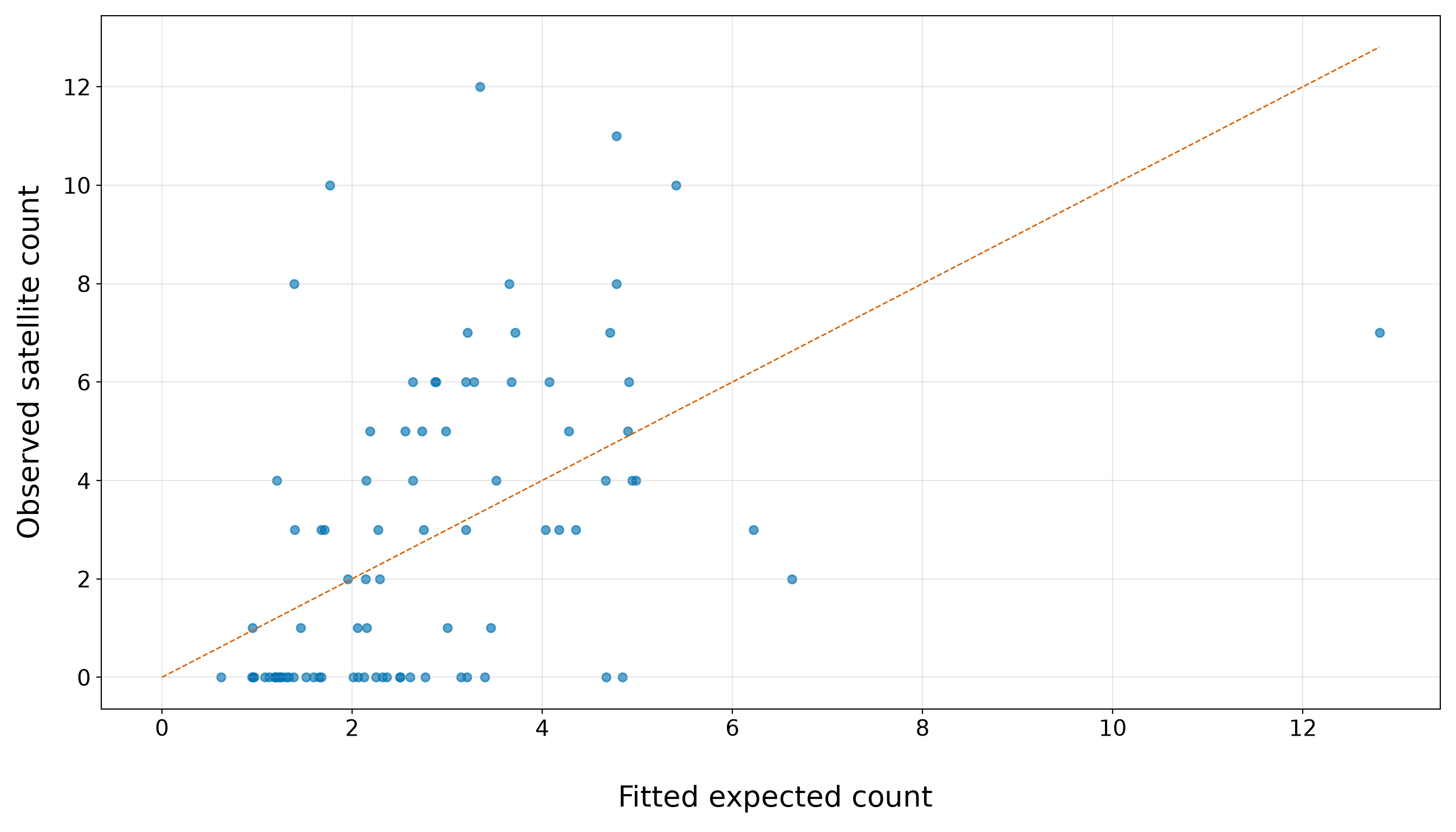
In Figure 10.16, the dashed line marks where the observed satellite count would equal the fitted expected count. Points above the line correspond to female crabs whose observed counts are larger than the extended model expects, while points below the line correspond to female crabs whose observed counts are smaller than expected. The plot shows that the extended model still has important calibration problems. Many observations with fitted expected counts between roughly \(1.5\) and \(4\) have observed counts of \(0\), so they sit well below the dashed line. This agrees with the grouped calibration in Table 10.42: the extended model continues to underestimate the frequency of zero satellite counts. At the same time, several observations in the same fitted-count range have observed counts around \(6\), \(8\), \(10\), or even \(12\), placing them far above the dashed line.
The horizontal bands are expected because the observed response is a count. The fitted expected count on the \(x\)-axis is allowed to be fractional, but the observed satellite count on the \(y\)-axis can only take values such as \(0, 1, 2, 3\), and so on. What is concerning is not the banding itself, but the wide vertical spread among observations with similar fitted expected counts.
Thus, the extended model captures some ordering in the mean structure, but it still struggles to reproduce the full spread of the training counts. The same fitted-count region contains many zeros and several large counts, which is exactly the kind of pattern that can produce both excess-zero concerns and overdispersion. This plot therefore provides a visual bridge to the more formal overdispersion, zero-count, and residual deviance checks below.
Extended Overdispersion Check
We first revisit overdispersion from Section 10.8.2. Recall that the Pearson dispersion estimate \(\hat{\phi}_P\) compares the Pearson Chi-squared statistic, from Equation 10.14, with the residual degrees of freedom (see Equation 10.15). Moreover, in this goodness-of-fit check for a one-sided test, the hypotheses for the dispersion term are:
\[ H_0\text{: } \phi = 1 \qquad\text{versus}\qquad H_1\text{: } \phi > 1. \]
Values of \(\phi\) much larger than \(1\) indicate that the observed counts vary more than the Classical Poisson model allows.
extended_pearson_chi_square <- sum(
  residuals(
    extended_poisson_model,
    type = "pearson"
  )^2
)

extended_pearson_df <- df.residual(extended_poisson_model)

extended_pearson_dispersion <- (
  extended_pearson_chi_square / extended_pearson_df
)

extended_overdispersion_p_value <- pchisq(
  extended_pearson_chi_square,
  df = extended_pearson_df,
  lower.tail = FALSE
)

extended_overdispersion_summary <- tibble::tibble(
  `Pearson Chi-squared statistic` = extended_pearson_chi_square,
  `Residual degrees of freedom` = extended_pearson_df,
  `Pearson dispersion estimate` = extended_pearson_dispersion,
  `Overdispersion p-value` = extended_overdispersion_p_value
) |>
  mutate(
    `Pearson Chi-squared statistic` = formatC(
      `Pearson Chi-squared statistic`,
      format = "f",
      digits = 3
    ),
    `Residual degrees of freedom` = formatC(
      `Residual degrees of freedom`,
      format = "f",
      digits = 0
    ),
    `Pearson dispersion estimate` = formatC(
      `Pearson dispersion estimate`,
      format = "f",
      digits = 3
    ),
    `Overdispersion p-value` = formatC(
      `Overdispersion p-value`,
      format = "e",
      digits = 2
    )
  ) |>
  pivot_longer(
    cols = everything(),
    names_to = "Quantity",
    values_to = "Value"
  )

extended_overdispersion_summary |>
  kable(
    align = c("c", "c")
)| Quantity | Value |
|---|---|
| Pearson Chi-squared statistic | 240.380 |
| Residual degrees of freedom | 78 |
| Pearson dispersion estimate | 3.082 |
| Overdispersion p-value | 1.91e-18 |
extended_pearson_chi_square = np.sum(
    extended_poisson_model.resid_pearson ** 2
)

extended_pearson_df = extended_poisson_model.df_resid

extended_pearson_dispersion = (
    extended_pearson_chi_square / extended_pearson_df
)

extended_overdispersion_p_value = stats.chi2.sf(
    extended_pearson_chi_square,
    extended_pearson_df
)

extended_overdispersion_summary = pd.DataFrame(
    {
        "Quantity": [
            "Pearson Chi-squared statistic",
            "Residual degrees of freedom",
            "Pearson dispersion estimate",
            "Overdispersion p-value",
        ],
        "Value": [
            f"{extended_pearson_chi_square:.3f}",
            f"{extended_pearson_df:.0f}",
            f"{extended_pearson_dispersion:.3f}",
            f"{extended_overdispersion_p_value:.2e}",
        ],
    }
)

classical_poisson_extended_overdispersion_py_html = (
    extended_overdispersion_summary.to_html(
        index=False,
        border=0,
    )
)| Quantity | Value |
|---|---|
| Pearson Chi-squared statistic | 240.380 |
| Residual degrees of freedom | 78 |
| Pearson dispersion estimate | 3.082 |
| Overdispersion p-value | 1.91e-18 |
For the extended model, the Pearson dispersion estimate is 3.082, with an overdispersion \(p\)-value of 1.91e-18. Since the dispersion estimate is still far above \(1\), the extended model continues to show substantial overdispersion relative to the Classical Poisson mean-variance assumption.
This means that adding weight, colour, and spine condition did not resolve the main variance problem. The training counts are still much more variable than the fitted Classical Poisson model allows. As a result, the model-based standard errors from this extended Poisson model still require caution because they rely on equidispersion. If used without adjustment, they may be too small, making Wald statistics too large, confidence intervals too narrow, and Type I errors more probable.
Extended Zero-Count Check

Next, we check whether the extended model expects enough zero counts as in Section 10.8.3. This is important because the simple width-only model substantially understated the number of zero satellite counts in the training data. Recall that this diagnostic focuses on the number of observed zero counts,
\[ z_{\operatorname{obs}} = \sum_{i=1}^n \mathbb{1}(y_i = 0), \]
where \(\mathbb{1}(y_i = 0)\) is an indicator that equals \(1\) when the \(i\)th observed satellite count is zero and equals \(0\) otherwise. Furthermore, in this goodness-of-fit check for a one-sided test, the hypotheses are:
\[ \begin{gather} H_0\text{: } \text{the fitted Classical Poisson model adequately describes} \\ \text{the frequency of zero counts}, \\ \text{versus} \\ H_1\text{: } \text{there are more zero counts than the} \\ \text{fitted Classical Poisson model expects}, \end{gather} \]
with an approximate \(z\)-statistic as in Equation 10.16.
extended_observed_zero_count <- sum(
  extended_poisson_gof_data$satellites == 0
)

extended_expected_zero_count <- sum(
  extended_poisson_gof_data$fitted_zero_probability
)

extended_zero_count_variance <- sum(
  extended_poisson_gof_data$fitted_zero_probability *
    (1 - extended_poisson_gof_data$fitted_zero_probability)
)

extended_zero_count_z <- (
  extended_observed_zero_count - extended_expected_zero_count
) / sqrt(extended_zero_count_variance)

extended_zero_count_p_value <- pnorm(
  extended_zero_count_z,
  lower.tail = FALSE
)

extended_zero_count_summary <- tibble::tibble(
  `Observed zero count` = extended_observed_zero_count,
  `Fitted expected zero count` = extended_expected_zero_count,
  `Observed minus fitted zeros` = (
    extended_observed_zero_count - extended_expected_zero_count
  ),
  `Zero-count z-statistic` = extended_zero_count_z,
  `Zero-count p-value` = extended_zero_count_p_value
) |>
  mutate(
    `Observed zero count` = formatC(
      `Observed zero count`,
      format = "f",
      digits = 0
    ),
    `Fitted expected zero count` = formatC(
      `Fitted expected zero count`,
      format = "f",
      digits = 2
    ),
    `Observed minus fitted zeros` = formatC(
      `Observed minus fitted zeros`,
      format = "f",
      digits = 2
    ),
    `Zero-count z-statistic` = formatC(
      `Zero-count z-statistic`,
      format = "f",
      digits = 2
    ),
    `Zero-count p-value` = formatC(
      `Zero-count p-value`,
      format = "e",
      digits = 2
    )
  ) |>
  pivot_longer(
    cols = everything(),
    names_to = "Quantity",
    values_to = "Value"
  )

extended_zero_count_summary |>
  kable(
    align = c("c", "c")
)| Quantity | Value |
|---|---|
| Observed zero count | 34 |
| Fitted expected zero count | 10.75 |
| Observed minus fitted zeros | 23.25 |
| Zero-count z-statistic | 8.15 |
| Zero-count p-value | 1.81e-16 |
extended_observed_zero_count = (
    extended_poisson_gof_data["satellites"] == 0
).sum()

extended_expected_zero_count = (
    extended_poisson_gof_data["fitted_zero_probability"].sum()
)

extended_zero_count_variance = (
    extended_poisson_gof_data["fitted_zero_probability"]
    * (1 - extended_poisson_gof_data["fitted_zero_probability"])
).sum()

extended_zero_count_z = (
    extended_observed_zero_count - extended_expected_zero_count
) / np.sqrt(extended_zero_count_variance)

extended_zero_count_p_value = stats.norm.sf(
    extended_zero_count_z
)

extended_zero_count_summary = pd.DataFrame(
    {
        "Quantity": [
            "Observed zero count",
            "Fitted expected zero count",
            "Observed minus fitted zeros",
            "Zero-count z-statistic",
            "Zero-count p-value",
        ],
        "Value": [
            f"{extended_observed_zero_count:.0f}",
            f"{extended_expected_zero_count:.2f}",
            f"{extended_observed_zero_count - extended_expected_zero_count:.2f}",
            f"{extended_zero_count_z:.2f}",
            f"{extended_zero_count_p_value:.2e}",
        ],
    }
)

classical_poisson_extended_zero_count_py_html = (
    extended_zero_count_summary.to_html(
        index=False,
        border=0,
    )
)| Quantity | Value |
|---|---|
| Observed zero count | 34 |
| Fitted expected zero count | 10.75 |
| Observed minus fitted zeros | 23.25 |
| Zero-count z-statistic | 8.15 |
| Zero-count p-value | 1.81e-16 |
The extended model still shows a substantial zero-count mismatch. In the training data, we observe 34 female crabs with zero satellite males, but the fitted extended Classical Poisson model expects only 10.75 zeros. This leaves 23.25 additional observed zeros beyond what the fitted model expects. Moreover, the approximate zero-count \(z\)-statistic is 8.15, with a one-sided \(p\)-value of 1.81e-16. This provides strong evidence that the extended model is still understating the zero-count part of the response distribution.
Compared with the simple width-only model, adding weight, colour, and spine condition gives the fitted mean structure more flexibility. However, the extended Classical Poisson model still expects far fewer zero satellite counts than we actually observe. This suggests that the remaining problem is not only that the systematic component was too simple; the Classical Poisson distribution itself is struggling to represent how often zero satellite counts occur in these training data.
Extended Residual Deviance Check
Finally, we revisit residual deviance as a global likelihood-based goodness-of-fit check from Section 10.8.4. This diagnostic, as in Equation 10.18, asks whether the extended model is still far from the saturated benchmark. Recall that the hypotheses are the following:
\[ \begin{gather} H_0\text{: } \text{the fitted Classical Poisson model is adequate}, \\ \text{versus} \\ H_1\text{: } \text{the fitted Classical Poisson model is not adequate}. \end{gather} \]
extended_residual_deviance <- deviance(extended_poisson_model)

extended_residual_deviance_df <- df.residual(extended_poisson_model)

extended_residual_deviance_ratio <- (
  extended_residual_deviance / extended_residual_deviance_df
)

extended_residual_deviance_p_value <- pchisq(
  extended_residual_deviance,
  df = extended_residual_deviance_df,
  lower.tail = FALSE
)

extended_residual_deviance_summary <- tibble::tibble(
  `Residual deviance` = extended_residual_deviance,
  `Residual degrees of freedom` = extended_residual_deviance_df,
  `Residual deviance / df` = extended_residual_deviance_ratio,
  `Goodness-of-fit p-value` = extended_residual_deviance_p_value
) |>
  mutate(
    `Residual deviance` = formatC(
      `Residual deviance`,
      format = "f",
      digits = 3
    ),
    `Residual degrees of freedom` = formatC(
      `Residual degrees of freedom`,
      format = "f",
      digits = 0
    ),
    `Residual deviance / df` = formatC(
      `Residual deviance / df`,
      format = "f",
      digits = 3
    ),
    `Goodness-of-fit p-value` = formatC(
      `Goodness-of-fit p-value`,
      format = "e",
      digits = 2
    )
  ) |>
  pivot_longer(
    cols = everything(),
    names_to = "Quantity",
    values_to = "Value"
  )

extended_residual_deviance_summary |>
  kable(
    align = c("c", "c")
)| Quantity | Value |
|---|---|
| Residual deviance | 248.028 |
| Residual degrees of freedom | 78 |
| Residual deviance / df | 3.180 |
| Goodness-of-fit p-value | 1.35e-19 |
extended_residual_deviance = extended_poisson_model.deviance

extended_residual_deviance_df = extended_poisson_model.df_resid

extended_residual_deviance_ratio = (
    extended_residual_deviance / extended_residual_deviance_df
)

extended_residual_deviance_p_value = stats.chi2.sf(
    extended_residual_deviance,
    extended_residual_deviance_df
)

extended_residual_deviance_summary = pd.DataFrame(
    {
        "Quantity": [
            "Residual deviance",
            "Residual degrees of freedom",
            "Residual deviance / df",
            "Goodness-of-fit p-value",
        ],
        "Value": [
            f"{extended_residual_deviance:.3f}",
            f"{extended_residual_deviance_df:.0f}",
            f"{extended_residual_deviance_ratio:.3f}",
            f"{extended_residual_deviance_p_value:.2e}",
        ],
    }
)

classical_poisson_extended_residual_deviance_py_html = (
    extended_residual_deviance_summary.to_html(
        index=False,
        border=0,
    )
)| Quantity | Value |
|---|---|
| Residual deviance | 248.028 |
| Residual degrees of freedom | 78 |
| Residual deviance / df | 3.180 |
| Goodness-of-fit p-value | 1.35e-19 |
For the extended model, the residual deviance is 248.028, with 78 residual degrees of freedom. The ratio of residual deviance to degrees of freedom is 3.180, which is still far above \(1\). This means that, even after adding weight, colour, and spine condition, the fitted extended Classical Poisson model remains much farther from the saturated benchmark than we would expect under an adequate model.
The corresponding goodness-of-fit \(p\)-value is 1.35e-19, providing strong global evidence of lack of fit. This agrees with the targeted diagnostics above: the extended model still shows substantial overdispersion and still expects far fewer zero satellite counts than observed. Taken together, these checks suggest that the issue is not only an incomplete set of regressors. The Classical Poisson distributional assumptions remain too restrictive for these training data.
Now, to see where some of the remaining lack of fit may be appearing, we can also inspect Pearson residuals against fitted expected counts for the extended model. This mirrors the diagnostic plot used for the simple width-only model in Section 10.8.4.
extended_pearson_residual_plot <- ggplot(
  extended_poisson_gof_data,
  aes(x = fitted_expected_count, y = pearson_residual)
) +
  geom_hline(
    yintercept = 0,
    linetype = "solid",
    linewidth = 0.8,
    colour = "grey40"
  ) +
  geom_hline(
    yintercept = c(-2, 2),
    linetype = "dashed",
    linewidth = 0.8,
    colour = "#D55E00"
  ) +
  geom_point(
    alpha = 0.65,
    size = 2.3,
    colour = "#0072B2"
  ) +
  theme_bw() +
  theme(
    axis.text = element_text(size = 15.5),
    axis.title.x = element_text(size = 20),
    axis.title.y = element_text(
      size = 20,
      vjust = 0.5,
      margin = margin(r = 12)
    ),
    panel.grid.minor = element_blank()
  ) +
  labs(
    x = "\n Fitted expected count",
    y = "Pearson residual"
  )

extended_pearson_residual_plot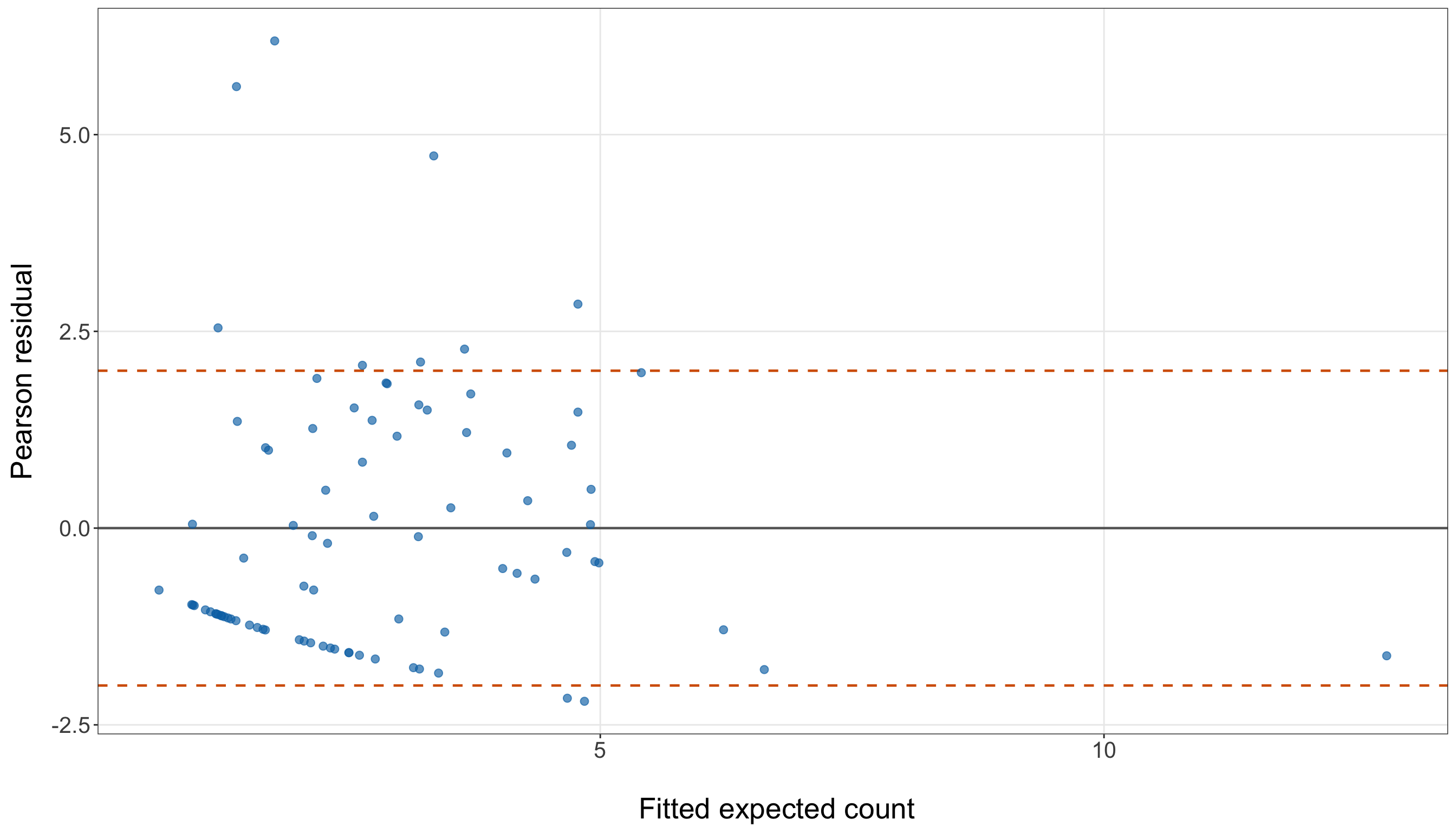
extended_pearson_residual_figure, extended_pearson_residual_axis = (
    plt.subplots(
        figsize=(14, 8)
    )
)

extended_pearson_residual_axis.axhline(
    0,
    linestyle="-",
    linewidth=0.8,
    color="grey"
)

extended_pearson_residual_axis.axhline(
    2,
    linestyle="--",
    linewidth=0.8,
    color="#D55E00"
)

extended_pearson_residual_axis.axhline(
    -2,
    linestyle="--",
    linewidth=0.8,
    color="#D55E00"
)

extended_pearson_residual_axis.scatter(
    extended_poisson_gof_data["fitted_expected_count"],
    extended_poisson_gof_data["pearson_residual"],
    alpha=0.65,
    s=35,
    color="#0072B2"
)

extended_pearson_residual_axis.set_xlabel(
    "\n Fitted expected count",
    fontsize=20
)

extended_pearson_residual_axis.set_ylabel(
    "Pearson residual",
    fontsize=20,
    labelpad=12
)

extended_pearson_residual_axis.tick_params(
    axis="both",
    labelsize=15.5
)

extended_pearson_residual_axis.grid(
    True,
    which="major",
    axis="both",
    alpha=0.3
)

extended_pearson_residual_axis.grid(
    False,
    which="minor"
)

extended_pearson_residual_figure.tight_layout()
plt.show()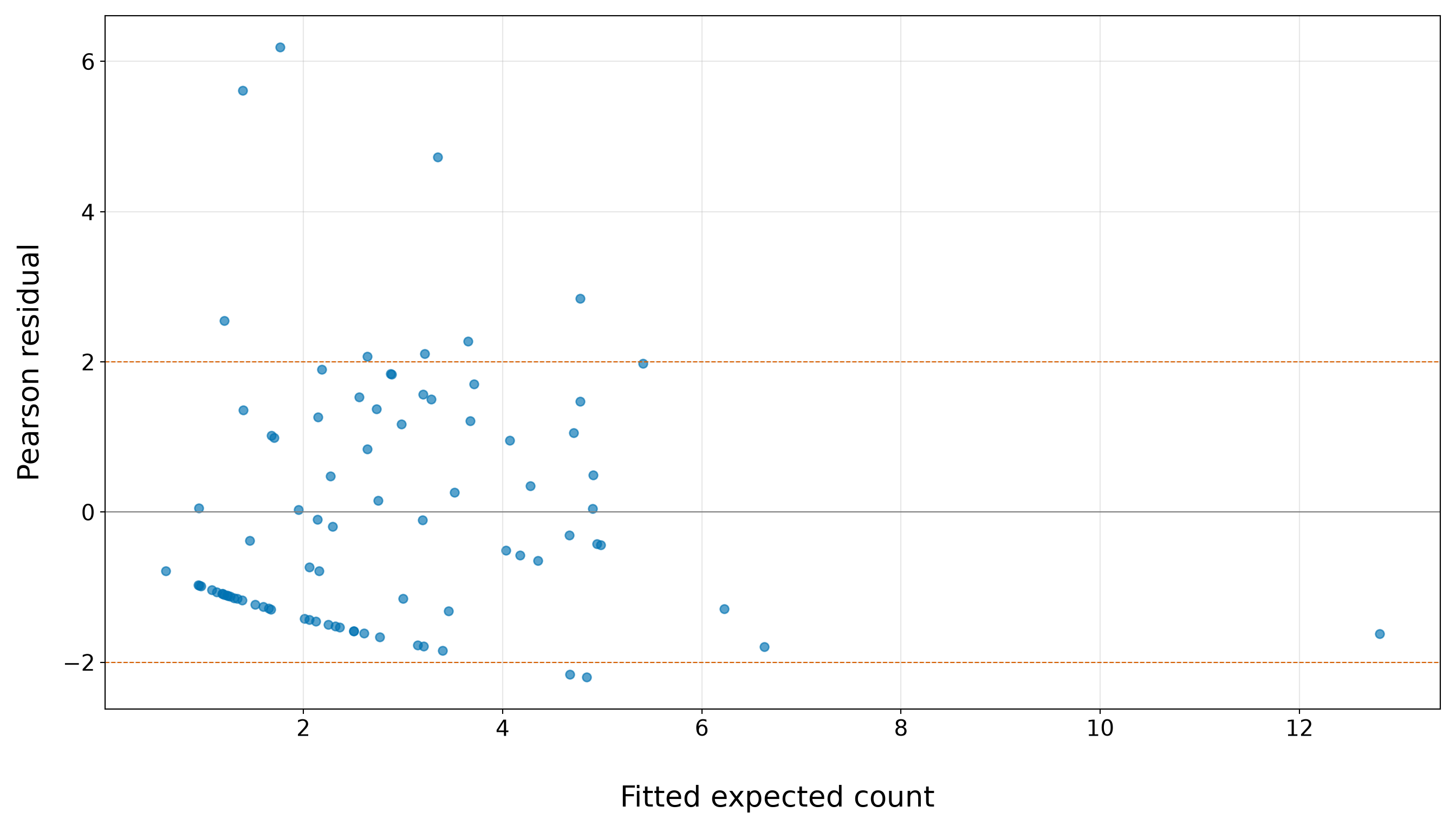
In Figure 10.18 (or Figure 10.19), the solid horizontal line at \(0\) marks where the observed count equals the fitted expected count after standardizing by the fitted Poisson standard deviation. The dashed horizontal lines at \(-2\) and \(2\) are informal reference bands for large Pearson residuals. They are not formal cutoffs, but they help us identify observations that are unusually far from the fitted model on the Poisson residual scale.
Having said that, the extended model still shows a clear residual pattern. Many observations with fitted expected counts between roughly \(1.5\) and \(5\) have negative Pearson residuals, forming a visible lower band below \(0\). These are female crabs whose observed satellite counts are smaller than the model expects, often corresponding to zero or very small observed counts. This pattern is consistent with the earlier zero-count diagnostic: even after adding weight, colour, and spine condition, the model still expects fewer zero satellite counts than we observe in the training data.

At the same time, several observations have positive Pearson residuals above \(2\), including a few very large residuals above \(5\). These are female crabs whose observed satellite counts are much larger than the extended model expects, even after accounting for the fitted Poisson standard deviation. Thus, the model is struggling in both directions: it underestimates the frequency of zeros for some observations while also failing to accommodate some unusually large satellite counts.
This plot helps explain why the extended Pearson dispersion and residual deviance diagnostics remain problematic. The issue is not only a single outlying crab or a small local pattern. The residuals show a wide vertical spread among observations with similar fitted expected counts, which is exactly the kind of pattern we would expect when the Classical Poisson mean-variance structure is too restrictive. Adding phenotypic regressors improves the systematic component, but it does not fully address the remaining distributional mismatch in these training data.
Extended Goodness-of-Fit Summary

The extended-model diagnostics are summarized in Table 10.50. This table brings together the main evidence from the observed-versus-fitted comparison, the Pearson overdispersion check, the zero-count check, and the residual deviance check.
| Diagnostic | Main evidence | Conclusion |
|---|---|---|
| Observed versus fitted counts | Observed zero proportions exceed fitted zero probabilities across the fitted-count quartiles. In Q1, the observed zero proportion is 0.773, while the average fitted probability of zero satellites is 0.307. In Q4, the observed zero proportion is 0.095, while the average fitted probability of zero satellites is 0.01. | The extended model captures some ordering in the fitted mean structure, but it still understates zero counts across the fitted-count range. |
| Pearson overdispersion | The Pearson dispersion estimate is 3.082, with an overdispersion \(p\)-value of 1.91e-18. | The training counts remain much more variable than the Classical Poisson mean-variance structure allows. |
| Excess zero counts | The training data contain 34 observed zero satellite counts, while the fitted extended model expects only 10.75 zeros. The zero-count \(p\)-value is 1.81e-16. | The extended model still expects far fewer zero satellite counts than observed in the training data. |
| Residual deviance | The residual deviance divided by its degrees of freedom is 3.180, with a goodness-of-fit \(p\)-value of 1.35e-19. | The extended model remains far from the saturated benchmark, giving global evidence of lack of fit. |
Overall, the extended model gives us a more complete fitted mean structure than the simple width-only model because it includes width, weight, colour, and spine condition. The observed-versus-fitted comparison shows that the extended model captures some broad ordering in the expected counts: observations in higher fitted-count quartiles tend to have larger mean observed counts. However, this improvement is not enough to make the Classical Poisson model adequate.
The main diagnostic problems remain:
- The Pearson dispersion estimate is 3.082, which is still far above \(1\), indicating substantial overdispersion.
- The zero-count check is also highly concerning: the training data contain 34 zero satellite counts, while the extended model expects only 10.75 zeros.
- The residual deviance ratio is 3.180, with a goodness-of-fit \(p\)-value of 1.35e-19, giving global evidence of lack of fit.
Thus, adding the phenotypic regressors improved the systematic component, but it did not resolve the distributional mismatch. The extended Classical Poisson model still struggles with both too much variability and too many zero counts relative to what the model expects. In practical terms, this means the fitted mean structure can still be useful for illustrating Poisson regression, but the Classical Poisson assumptions are not adequate enough to treat this model as a fully satisfactory final model.
For learning purposes, we continue with the extended Classical Poisson model so that we can show how coefficient interpretation and prediction work in a Poisson GLM. The diagnostic concerns should remain visible, though. They are not side notes; they explain why later count-regression chapters consider alternatives such as Negative Binomial regression (Chapter 11) for overdispersed counts and Zero-Inflated Poisson regression (Chapter 12) for zero-heavy count responses.
10.9.3 Interpreting Continuous Regressors
We now interpret the continuous regressors in the extended model. The key point is that the log link makes coefficient interpretation multiplicative on the expected-count scale. From Equation 10.19 in this extended model, recall that the modelling equation is
\[ \log(\mu_i) = \beta_0 + \beta_1 x_{i,1} + \beta_2 x_{i,2} + \beta_3 x_{i,3} + \cdots + \beta_7 x_{i,7}, \]
where \(x_{i,1}\) is female crab width in centimetres and \(x_{i,2}\) is female crab weight in kilograms.
For the continuous regressor \(x_{i,1}\), the coefficient is \(\beta_1\). To interpret it, compare two female crabs that have the same values of \(x_{i,2}, x_{i,3}, \ldots, x_{i,7}\), but whose widths differ by one centimetre. That is, compare one crab with width \(x_{i,1}\) to another otherwise comparable crab with width \(x_{i,1}+1\). For the crab with width \(x_{i,1}\), from Equation 10.20, the expected count is
\[ \mu(x_{i,1}) = \exp\left( \beta_0 + \beta_1 x_{i,1} + \beta_2 x_{i,2} + \cdots + \beta_7 x_{i,7} \right). \]
For the otherwise comparable crab with width \(x_{i,1}+1\), the expected count is
\[ \mu(x_{i,1}+1) = \exp\left[ \beta_0 + \beta_1(x_{i,1}+1) + \beta_2 x_{i,2} + \cdots + \beta_7 x_{i,7} \right]. \]
Taking the ratio gives
\[ \frac{ \mu(x_{i,1}+1) }{ \mu(x_{i,1}) } = \frac{ \exp\left[ \beta_0 + \beta_1(x_{i,1}+1) + \beta_2 x_{i,2} + \cdots + \beta_7 x_{i,7} \right] }{ \exp\left( \beta_0 + \beta_1 x_{i,1} + \beta_2 x_{i,2} + \cdots + \beta_7 x_{i,7} \right) }. \]
After cancellation, this becomes
\[ \frac{ \mu(x_{i,1}+1) }{ \mu(x_{i,1}) } = \exp(\beta_1). \]
Thus, \(\exp(\beta_1)\) is the multiplicative change in the expected number of satellite males for a one-centimetre increase in female crab width, holding weight, colour, and spine condition fixed. The corresponding percent change is
\[ \left[ \exp(\beta_1) - 1 \right] \times 100\%. \]
For the continuous regressor \(x_{i,2}\), the coefficient is \(\beta_2\). The interpretation is analogous. Compare two female crabs that have the same values of \(x_{i,1}, x_{i,3}, \ldots, x_{i,7}\), but whose weights differ by one kilogram. That is, compare one crab with weight \(x_{i,2}\) to another otherwise comparable crab with weight \(x_{i,2}+1\).
The expected-count ratio is
\[ \frac{ \mu(x_{i,2}+1) }{ \mu(x_{i,2}) } = \exp(\beta_2). \]
Thus, \(\exp(\beta_2)\) is the multiplicative change in the expected number of satellite males for a one-kilogram increase in female crab weight, holding width, colour, and spine condition fixed. The corresponding percent change is
\[ \left[ \exp(\beta_2) - 1 \right] \times 100\%. \]
Heads-up on holding other regressors fixed!
The phrase “holding other regressors fixed” is essential in the extended model. The coefficient for \(x_{i,1}\) describes a width comparison among female crabs with the same weight, colour category, and spine condition in the model. The coefficient for \(x_{i,2}\) describes a weight comparison among female crabs with the same width, colour category, and spine condition in the model.

This does not mean that the dataset literally contains pairs of crabs that are identical on all other variables. It means that the regression coefficient is interpreted conditionally within the model’s systematic component.
Table 10.51 extracts the continuous-regressor interpretations from the extended model.
continuous_interpretation <- extended_poisson_summary |>
  filter(
    term %in% c("width_cm", "weight_kg")
  ) |>
  mutate(
    notation = case_when(
      term == "width_cm" ~ "$x_{i,1}$",
      term == "weight_kg" ~ "$x_{i,2}$",
      TRUE ~ term
    ),
    interpretation_unit = case_when(
      term == "width_cm" ~ "One-centimetre increase in width",
      term == "weight_kg" ~ "One-kilogram increase in weight",
      TRUE ~ term
    )
  ) |>
  transmute(
    notation,
    interpretation_unit,
    estimate,
    exponentiated_estimate,
    percent_change
  )

continuous_interpretation |>
  rename(
    `Notation` = notation,
    `Comparison` = interpretation_unit,
    `Log-scale estimate` = estimate,
    `Multiplicative change in expected count` = exponentiated_estimate,
    `Percent change in expected count` = percent_change
  ) |>
  kable(
    align = c("c", "c", "c", "c", "c"),
    escape = FALSE
)| Notation | Comparison | Log-scale estimate | Multiplicative change in expected count | Percent change in expected count |
|---|---|---|---|---|
| \(x_{i,1}\) | One-centimetre increase in width | 0.05 | 1.05 | 4.60 |
| \(x_{i,2}\) | One-kilogram increase in weight | 0.58 | 1.79 | 79.42 |
continuous_interpretation = (
    extended_poisson_summary
    .query("Term in ['width_cm', 'weight_kg']")
    [
        [
            "Term",
            "Estimate",
            "Exponentiated estimate",
            "Percent change",
        ]
    ]
    .copy()
)

continuous_interpretation["Notation"] = (
    continuous_interpretation["Term"]
    .replace(
        {
            "width_cm": "$x_{i,1}$",
            "weight_kg": "$x_{i,2}$",
        }
    )
)

continuous_interpretation["Comparison"] = (
    continuous_interpretation["Term"]
    .replace(
        {
            "width_cm": "One-centimetre increase in width",
            "weight_kg": "One-kilogram increase in weight",
        }
    )
)

continuous_interpretation_display = continuous_interpretation[
    [
        "Notation",
        "Comparison",
        "Estimate",
        "Exponentiated estimate",
        "Percent change",
    ]
].rename(
    columns={
        "Estimate": "Log-scale estimate",
        "Exponentiated estimate": (
            "Multiplicative change in expected count"
        ),
        "Percent change": "Percent change in expected count",
    }
)

classical_poisson_continuous_interpretation_py_html = (
    continuous_interpretation_display.to_html(
        index=False,
        border=0,
        escape=False,
    )
)| Notation | Comparison | Log-scale estimate | Multiplicative change in expected count | Percent change in expected count |
|---|---|---|---|---|
| \(x_{i,1}\) | One-centimetre increase in width | 0.05 | 1.05 | 4.60 |
| \(x_{i,2}\) | One-kilogram increase in weight | 0.58 | 1.79 | 79.42 |
From Table 10.51, note the following:
- For \(x_{i,1}\), the fitted multiplicative change is 1.05. This means that, holding weight, colour, and spine condition fixed, increasing female crab width by one centimetre is associated with multiplying the expected number of satellite males by this value under the extended Classical Poisson model. The percent-change version is 4.6%.
- For \(x_{i,2}\), the fitted multiplicative change is 1.79. This means that, holding width, colour, and spine condition fixed, increasing female crab weight by one kilogram is associated with multiplying the expected number of satellite males by this value. The percent-change version is 79.42%.
Because one kilogram is a large change for female crabs in this dataset, we should be careful not to compare the magnitude of the width and weight coefficients without considering their measurement units and the overlap between body-size measurements.
10.9.4 Interpreting Categorical Regressors
Categorical regressors are interpreted through their dummy variables. In this extended model via Equation 10.19, colour is represented by \(x_{i,3}\), \(x_{i,4}\), and \(x_{i,5}\), with Light as the reference category. Spine condition is represented by \(x_{i,6}\) and \(x_{i,7}\), with Both good as the reference category. Table 10.39 illustrates the whole dummy variable arrangement.
Consider the dummy regressor \(x_{i,3}\) for Medium light colour. Holding width, weight, and spine condition fixed, this coefficient compares a female crab in the Medium light colour category with an otherwise comparable female crab in the Light reference category. For a crab in the Light reference category, the colour dummy variables satisfy
\[ x_{i,3}=x_{i,4}=x_{i,5}=0. \]
For an otherwise comparable crab in the Medium light category,
\[ x_{i,3}=1, \qquad x_{i,4}=0, \qquad x_{i,5}=0. \]
Therefore, the difference in log expected counts between Medium light and Light, holding the other regressors fixed, is
\[ \log(\mu_{\texttt{Medium light}}) - \log(\mu_{\texttt{Light}}) = \beta_3. \]
Equivalently,
\[ \frac{ \mu_{\texttt{Medium light}} }{ \mu_{\texttt{Light}} } = \exp(\beta_3). \]
The same logic applies to the other dummy variables. In general, for a dummy regressor \(x_{i,j}\), the exponentiated coefficient \(\exp(\beta_j)\) is the multiplicative comparison between the expected count in the category represented by that dummy variable and the expected count in the reference category, holding the other regressors fixed.
The corresponding percent difference is
\[ \left[ \exp(\beta_j) - 1 \right] \times 100\%. \]
Table 10.53 extracts the categorical-regressor interpretations.
categorical_interpretation <- extended_poisson_summary |>
  filter(
    !term %in% c("(Intercept)", "width_cm", "weight_kg")
  ) |>
  mutate(
    notation = case_when(
      term == "colorMedium light" ~ "$x_{i,3}$",
      term == "colorMedium dark" ~ "$x_{i,4}$",
      term == "colorDark" ~ "$x_{i,5}$",
      term == "spineOne worn or broken" ~ "$x_{i,6}$",
      term == "spineBoth worn or broken" ~ "$x_{i,7}$",
      TRUE ~ term
    ),
    comparison = case_when(
      term == "colorMedium light" ~ "Medium light versus Light",
      term == "colorMedium dark" ~ "Medium dark versus Light",
      term == "colorDark" ~ "Dark versus Light",
      term == "spineOne worn or broken" ~
        "One worn or broken versus Both good",
      term == "spineBoth worn or broken" ~
        "Both worn or broken versus Both good",
      TRUE ~ term
    )
  ) |>
  transmute(
    notation,
    comparison,
    estimate,
    exponentiated_estimate,
    percent_change
  )

categorical_interpretation |>
  rename(
    `Notation` = notation,
    `Category comparison` = comparison,
    `Log-scale estimate` = estimate,
    `Multiplicative change in expected count` = exponentiated_estimate,
    `Percent difference in expected count` = percent_change
  ) |>
  kable(
    align = c("c", "c", "c", "c", "c"),
    escape = FALSE
)| Notation | Category comparison | Log-scale estimate | Multiplicative change in expected count | Percent difference in expected count |
|---|---|---|---|---|
| \(x_{i,3}\) | Medium light versus Light | -0.35 | 0.71 | -29.45 |
| \(x_{i,4}\) | Medium dark versus Light | -0.48 | 0.62 | -38.22 |
| \(x_{i,5}\) | Dark versus Light | -0.86 | 0.42 | -57.54 |
| \(x_{i,6}\) | One worn or broken versus Both good | 0.00 | 1.00 | 0.06 |
| \(x_{i,7}\) | Both worn or broken versus Both good | 0.51 | 1.66 | 66.43 |
categorical_interpretation = extended_poisson_summary[
    ~extended_poisson_summary["Term"].isin(
        [
            "Intercept",
            "width_cm",
            "weight_kg",
        ]
    )
].copy()

notation_labels = {
    (
        "C(color, Treatment(reference='Light'))"
        "[T.Medium light]"
    ): "$x_{i,3}$",
    (
        "C(color, Treatment(reference='Light'))"
        "[T.Medium dark]"
    ): "$x_{i,4}$",
    (
        "C(color, Treatment(reference='Light'))"
        "[T.Dark]"
    ): "$x_{i,5}$",
    (
        "C(spine, Treatment(reference='Both good'))"
        "[T.One worn or broken]"
    ): "$x_{i,6}$",
    (
        "C(spine, Treatment(reference='Both good'))"
        "[T.Both worn or broken]"
    ): "$x_{i,7}$",
}

comparison_labels = {
    (
        "C(color, Treatment(reference='Light'))"
        "[T.Medium light]"
    ): "Medium light versus Light",
    (
        "C(color, Treatment(reference='Light'))"
        "[T.Medium dark]"
    ): "Medium dark versus Light",
    (
        "C(color, Treatment(reference='Light'))"
        "[T.Dark]"
    ): "Dark versus Light",
    (
        "C(spine, Treatment(reference='Both good'))"
        "[T.One worn or broken]"
    ): "One worn or broken versus Both good",
    (
        "C(spine, Treatment(reference='Both good'))"
        "[T.Both worn or broken]"
    ): "Both worn or broken versus Both good",
}

categorical_interpretation["Notation"] = (
    categorical_interpretation["Term"].replace(notation_labels)
)

categorical_interpretation["Category comparison"] = (
    categorical_interpretation["Term"].replace(comparison_labels)
)

categorical_interpretation_display = categorical_interpretation[
    [
        "Notation",
        "Category comparison",
        "Estimate",
        "Exponentiated estimate",
        "Percent change",
    ]
].rename(
    columns={
        "Estimate": "Log-scale estimate",
        "Exponentiated estimate": (
            "Multiplicative change in expected count"
        ),
        "Percent change": "Percent difference in expected count",
    }
)

classical_poisson_categorical_interpretation_py_html = (
    categorical_interpretation_display.to_html(
        index=False,
        border=0,
        escape=False,
    )
)| Notation | Category comparison | Log-scale estimate | Multiplicative change in expected count | Percent difference in expected count |
|---|---|---|---|---|
| \(x_{i,3}\) | Medium light versus Light | -0.35 | 0.71 | -29.45 |
| \(x_{i,4}\) | Medium dark versus Light | -0.48 | 0.62 | -38.22 |
| \(x_{i,5}\) | Dark versus Light | -0.86 | 0.42 | -57.54 |
| \(x_{i,6}\) | One worn or broken versus Both good | 0.00 | 1.00 | 0.06 |
| \(x_{i,7}\) | Both worn or broken versus Both good | 0.51 | 1.66 | 66.43 |
For a categorical regressor, an exponentiated estimate below \(1\) means that the comparison category has a smaller fitted expected count than the reference category, holding the other regressors fixed. On the other hand, an exponentiated estimate above \(1\) means that the comparison category has a larger fitted expected count than the reference category, holding the other regressors fixed.
Note that these are conditional, model-based comparisons. They describe the fitted mean structure of the extended Classical Poisson model, not final inferential conclusions. Since the extended model still shows overdispersion and excess zero counts, the coefficient interpretations should be read together with the goodness-of-fit results. Wald tests and final inferential claims are saved for the results section.
10.10 Prediction with Poisson Regression
Prediction with a fitted Poisson regression model means predicting the expected count for a new or held-out observation. For a new female crab with regressor row vector
\[ \mathbf{x}_{\operatorname{new}}^\top = \begin{bmatrix} 1 & x_{\operatorname{new},1} & x_{\operatorname{new},2} & \cdots & x_{\operatorname{new},7} \end{bmatrix}, \]
the fitted expected count is
\[ \hat{\mu}_{\operatorname{new}} = \exp \left( \mathbf{x}_{\operatorname{new}}^\top \hat{\boldsymbol{\beta}}_{\operatorname{MLE,obs}} \right). \]

In scalar notation,
\[ \hat{\mu}_{\operatorname{new}} = \exp \left( \hat{\beta}_{0,\operatorname{MLE,obs}} + \hat{\beta}_{1,\operatorname{MLE,obs}}x_{\operatorname{new},1} + \hat{\beta}_{2,\operatorname{MLE,obs}}x_{\operatorname{new},2} + \cdots + \hat{\beta}_{7,\operatorname{MLE,obs}}x_{\operatorname{new},7} \right). \]
This predicted value is on the response scale. It is an expected count, not a rounded count. Therefore, it can have decimal places but must be positive.
Heads-up on predicting counts versus predicting expected counts!
A Poisson regression model usually predicts the expected count \(\hat{\mu}_{\operatorname{new}}\), not the exact count that will be observed. The observed count is random and can take values \(0, 1, 2, \ldots\).
For example, a predicted expected count of \(3.4\) satellite males does not mean that the next observed count will be exactly \(3.4\). It means that, under the fitted model, the expected number of satellite males for female crabs with those regressor values is \(3.4\).
If we need a full predictive distribution, we can combine the fitted expected count with the Poisson distribution:
\[ Y_{\operatorname{new}} \mid x_{\operatorname{new},1}, x_{\operatorname{new},2}, \ldots, x_{\operatorname{new},7} \sim \operatorname{Poisson} \left( \hat{\mu}_{\operatorname{new}} \right). \]
The code below uses the extended model to create fitted expected counts for the held-out testing data. We are not summarizing prediction accuracy yet. The results section will use these predictions to evaluate predictive performance with held-out data.
extended_poisson_test_predictions <- testing_data |>
  mutate(
    predicted_expected_count = predict(
      extended_poisson_model,
      newdata = testing_data,
      type = "response"
    )
  ) |>
  select(
    satellites,
    width_cm,
    weight_kg,
    color,
    spine,
    predicted_expected_count
  ) |>
  slice_head(n = 10) |>
  mutate(
    predicted_expected_count = round(predicted_expected_count, 2)
  )

extended_poisson_test_predictions |>
  rename(
    `Observed satellite count` = satellites,
    `Female crab width (cm)` = width_cm,
    `Female crab weight (kg)` = weight_kg,
    `Colour` = color,
    `Spine condition` = spine,
    `Predicted expected count` = predicted_expected_count
  ) |>
  kable(
    align = c("c", "c", "c", "c", "c", "c")
)| Observed satellite count | Female crab width (cm) | Female crab weight (kg) | Colour | Spine condition | Predicted expected count |
|---|---|---|---|---|---|
| 8 | 28.3 | 3.05 | Medium light | Both worn or broken | 4.80 |
| 0 | 22.5 | 1.55 | Medium dark | Both worn or broken | 1.35 |
| 9 | 26.0 | 2.30 | Light | Both good | 2.38 |
| 4 | 26.0 | 2.60 | Medium dark | Both worn or broken | 2.91 |
| 0 | 24.7 | 1.90 | Medium dark | One worn or broken | 1.10 |
| 0 | 23.7 | 1.95 | Medium light | Both good | 1.23 |
| 0 | 25.6 | 2.15 | Medium dark | Both worn or broken | 2.20 |
| 0 | 24.3 | 2.15 | Medium dark | Both worn or broken | 2.07 |
| 14 | 26.0 | 2.30 | Medium light | Both good | 1.68 |
| 1 | 25.2 | 2.00 | Medium light | Both worn or broken | 2.26 |
extended_poisson_testing_data = testing_data.copy()

extended_poisson_testing_data["color"] = pd.Categorical(
    extended_poisson_testing_data["color"],
    categories=color_order
)

extended_poisson_testing_data["spine"] = pd.Categorical(
    extended_poisson_testing_data["spine"],
    categories=spine_order
)

extended_poisson_testing_data["predicted_expected_count"] = (
    extended_poisson_model.predict(extended_poisson_testing_data)
)

extended_poisson_test_predictions = (
    extended_poisson_testing_data
    [
        [
            "satellites",
            "width_cm",
            "weight_kg",
            "color",
            "spine",
            "predicted_expected_count",
        ]
    ]
    .head(10)
    .copy()
)

extended_poisson_test_predictions["predicted_expected_count"] = (
    extended_poisson_test_predictions["predicted_expected_count"].round(2)
)

extended_poisson_test_predictions_display = (
    extended_poisson_test_predictions
    .rename(
        columns={
            "satellites": "Observed satellite count",
            "width_cm": "Female crab width (cm)",
            "weight_kg": "Female crab weight (kg)",
            "color": "Colour",
            "spine": "Spine condition",
            "predicted_expected_count": "Predicted expected count",
        }
    )
)

classical_poisson_test_predictions_py_html = (
    extended_poisson_test_predictions_display.to_html(
        index=False,
        border=0,
    )
)| Observed satellite count | Female crab width (cm) | Female crab weight (kg) | Colour | Spine condition | Predicted expected count |
|---|---|---|---|---|---|
| 8.0 | 28.3 | 3.05 | Medium light | Both worn or broken | 4.80 |
| 0.0 | 22.5 | 1.55 | Medium dark | Both worn or broken | 1.35 |
| 9.0 | 26.0 | 2.30 | Light | Both good | 2.38 |
| 4.0 | 26.0 | 2.60 | Medium dark | Both worn or broken | 2.91 |
| 0.0 | 24.7 | 1.90 | Medium dark | One worn or broken | 1.10 |
| 0.0 | 23.7 | 1.95 | Medium light | Both good | 1.23 |
| 0.0 | 25.6 | 2.15 | Medium dark | Both worn or broken | 2.20 |
| 0.0 | 24.3 | 2.15 | Medium dark | Both worn or broken | 2.07 |
| 14.0 | 26.0 | 2.30 | Medium light | Both good | 1.68 |
| 1.0 | 25.2 | 2.00 | Medium light | Both worn or broken | 2.26 |
The above prediction code uses the same fitted model object estimated on the training data:
- In
R,type = "response"asks for predictions on the expected-count scale rather than the log scale. - In
Python, {statsmodels} returns fitted GLM predictions on the response scale by default for this call.
The held-out predictions are ready for Section 10.11. There, we will compare the observed testing counts with the predicted expected counts and summarize predictive performance. For now, the key point is that prediction in Classical Poisson regression passes through the same two-step structure as fitting: first compute the systematic score, then convert it to a positive expected count through the exponential function.
10.11 Results and Statistical Interpretation
Now, we move from model building to results. Up to this point, the training data have been used to explore the response, fit the simple and extended Classical Poisson regression models, and diagnose goodness of fit. The extended model gave us a richer fitted mean structure than the simple width-only model, but the diagnostics still showed substantial overdispersion, excess zero counts, and global lack of fit.
Recall that this chapter has two guiding inquiries as in Table 10.57.
| Inquiry type | Research question | What the Results section must deliver |
|---|---|---|
| Inferential inquiry | How is the expected number of satellite males associated with female crab width, weight, colour, and spine condition? | A coefficient-level statistical interpretation of the extended Classical Poisson model, using the testing-set refit. |
| Predictive inquiry | How accurately can female crab characteristics predict the number of satellite males for held-out crabs? | A held-out predictive assessment using the training-fitted extended model evaluated on the testing data. |

Therefore, the results stage has two complementary goals:
- For the inferential inquiry, we refit the extended Classical Poisson model on the testing data and summarize the coefficient-level results.
- For the predictive inquiry, we evaluate how well the training-fitted extended model predicts the held-out testing counts.
This separation follows the data science workflow used throughout the book. The training data supported model development and goodness-of-fit checks. The testing data are now used for final assessment: coefficient-level inferential summaries for the inferential inquiry, and held-out prediction accuracy for the predictive inquiry.
Heads-up on why the testing data appear in two roles here!
The testing data are used differently for the two workflow flavours:
- For the inferential inquiry, we refit the selected extended model on the testing data. This gives a final coefficient-level analysis on data that were not used for EDA, model development, or goodness-of-fit decisions.
- For the predictive inquiry, we do not refit the model before predicting. We use the extended model fitted on the training data to generate predictions for the testing observations, and then compare those predictions with the observed testing counts.
These two uses should not be mixed. Refitting on the testing data is appropriate for the final inferential summary under this chapter’s workflow. Predictive evaluation, however, must use predictions from a model trained before looking at the testing responses.
10.11.1 Inferential Results: Refit the Extended Model on the Testing Data
For the inferential inquiry, we refit the extended Classical Poisson model using the testing data. The model has the same systematic component developed earlier:
\[ Y_i \mid x_{i,1}, x_{i,2}, \ldots, x_{i,7} \sim \operatorname{Poisson}(\mu_i), \]
with
\[ \begin{align*} \log(\mu_i) &= \beta_0 + \beta_1 x_{i,1} + \beta_2 x_{i,2} + \beta_3 x_{i,3} + \\ & \beta_4 x_{i,4} + \beta_5 x_{i,5} + \beta_6 x_{i,6} + \beta_7 x_{i,7}. \end{align*} \tag{10.21}\]
In Equation 10.21, \(x_{i,1}\) is width, \(x_{i,2}\) is weight, \(x_{i,3}\), \(x_{i,4}\), and \(x_{i,5}\) are colour dummy variables, and \(x_{i,6}\) and \(x_{i,7}\) are spine-condition dummy variables (see Table 10.39).

Before interpreting the coefficients on the expected-count scale, we first refit the extended Classical Poisson model on the testing data. This refit uses the same model form selected during the training-stage workflow, but it is estimated using observations that were not used for EDA, model building, or goodness-of-fit decisions. Table 10.58 reports the coefficient estimates on the log expected-count scale. This is the scale on which the GLM is fitted and on which the Wald statistics are computed. The coefficient estimate tells us the estimated additive change in \(\log(\mu_i)\), the standard error measures uncertainty on that same scale, and the Wald statistic compares the estimate with the null value \(0\).
final_poisson_inference_model <- glm(
  satellites ~ width_cm + weight_kg + color + spine,
  family = poisson(link = "log"),
  data = testing_data
)

final_poisson_inference_summary <- tidy(
  final_poisson_inference_model
) |>
  mutate(
    conf_low = estimate - qnorm(0.975) * std.error,
    conf_high = estimate + qnorm(0.975) * std.error,
    exponentiated_estimate = exp(estimate),
    exponentiated_conf_low = exp(conf_low),
    exponentiated_conf_high = exp(conf_high),
    percent_change = 100 * (exponentiated_estimate - 1),
    across(
      where(is.numeric),
      ~ round(.x, 2)
    )
  )

final_poisson_inference_summary |>
  select(
    term,
    estimate,
    std.error,
    statistic,
    p.value
  ) |>
  rename(
    `Term` = term,
    `Log-scale estimate` = estimate,
    `Standard error` = std.error,
    `Wald statistic` = statistic,
    `p-value` = p.value
  ) |>
  kable(
    align = c("c", "c", "c", "c", "c")
)| Term | Log-scale estimate | Standard error | Wald statistic | p-value |
|---|---|---|---|---|
| (Intercept) | 0.37 | 1.56 | 0.24 | 0.81 |
| width_cm | 0.02 | 0.08 | 0.28 | 0.78 |
| weight_kg | 0.28 | 0.33 | 0.87 | 0.39 |
| colorMedium light | -0.37 | 0.25 | -1.50 | 0.13 |
| colorMedium dark | -0.75 | 0.29 | -2.58 | 0.01 |
| colorDark | -0.45 | 0.32 | -1.39 | 0.17 |
| spineOne worn or broken | -0.32 | 0.27 | -1.17 | 0.24 |
| spineBoth worn or broken | -0.22 | 0.16 | -1.36 | 0.17 |
final_poisson_inference_data = testing_data.copy()

final_poisson_inference_data["color"] = pd.Categorical(
    final_poisson_inference_data["color"],
    categories=color_order
)

final_poisson_inference_data["spine"] = pd.Categorical(
    final_poisson_inference_data["spine"],
    categories=spine_order
)

final_poisson_inference_model = smf.glm(
    formula=(
        "satellites ~ width_cm + weight_kg "
        "+ C(color, Treatment(reference='Light')) "
        "+ C(spine, Treatment(reference='Both good'))"
    ),
    data=final_poisson_inference_data,
    family=sm.families.Poisson()
).fit()

final_poisson_inference_summary = pd.DataFrame(
    {
        "Term": final_poisson_inference_model.params.index,
        "Log-scale estimate": final_poisson_inference_model.params.values,
        "Standard error": final_poisson_inference_model.bse.values,
        "Wald statistic": final_poisson_inference_model.tvalues.values,
        "p-value": final_poisson_inference_model.pvalues.values,
    }
)

final_poisson_inference_summary[
    "Lower 95% CI on log scale"
] = (
    final_poisson_inference_summary["Log-scale estimate"]
    - stats.norm.ppf(0.975)
    * final_poisson_inference_summary["Standard error"]
)

final_poisson_inference_summary[
    "Upper 95% CI on log scale"
] = (
    final_poisson_inference_summary["Log-scale estimate"]
    + stats.norm.ppf(0.975)
    * final_poisson_inference_summary["Standard error"]
)

final_poisson_inference_summary[
    "Exponentiated estimate"
] = np.exp(
    final_poisson_inference_summary["Log-scale estimate"]
)

final_poisson_inference_summary[
    "Lower 95% CI for exponentiated estimate"
] = np.exp(
    final_poisson_inference_summary["Lower 95% CI on log scale"]
)

final_poisson_inference_summary[
    "Upper 95% CI for exponentiated estimate"
] = np.exp(
    final_poisson_inference_summary["Upper 95% CI on log scale"]
)

final_poisson_inference_summary["Percent change"] = (
    100
    * (
        final_poisson_inference_summary["Exponentiated estimate"]
        - 1
    )
)

final_poisson_inference_log_scale_display = (
    final_poisson_inference_summary
    [
        [
            "Term",
            "Log-scale estimate",
            "Standard error",
            "Wald statistic",
            "p-value",
        ]
    ]
    .round(2)
)

classical_poisson_test_refit_log_scale_py_html = (
    final_poisson_inference_log_scale_display.to_html(
        index=False,
        border=0,
    )
)| Term | Log-scale estimate | Standard error | Wald statistic | p-value |
|---|---|---|---|---|
| Intercept | 0.37 | 1.56 | 0.24 | 0.81 |
| C(color, Treatment(reference=‘Light’))[T.Medium light] | -0.37 | 0.25 | -1.50 | 0.13 |
| C(color, Treatment(reference=‘Light’))[T.Medium dark] | -0.75 | 0.29 | -2.58 | 0.01 |
| C(color, Treatment(reference=‘Light’))[T.Dark] | -0.45 | 0.32 | -1.39 | 0.17 |
| C(spine, Treatment(reference=‘Both good’))[T.One worn or broken] | -0.32 | 0.27 | -1.17 | 0.24 |
| C(spine, Treatment(reference=‘Both good’))[T.Both worn or broken] | -0.22 | 0.16 | -1.36 | 0.17 |
| width_cm | 0.02 | 0.08 | 0.28 | 0.78 |
| weight_kg | 0.28 | 0.33 | 0.87 | 0.39 |
Table 10.58 reports the testing-set refit on the scale used by the model. For each coefficient, the Wald statistic is the ratio between the estimated coefficient and its model-based standard error. Therefore, large positive or negative Wald statistics indicate estimates that are far from \(0\) relative to their estimated uncertainty. However, the log expected-count scale is not always the easiest scale for substantive interpretation. Since the model uses a log link (see Equation 10.21), exponentiating a coefficient gives a multiplicative comparison on the expected-count scale (see Equation 10.20). Thus, Table 10.60 reports these exponentiated estimates, their approximate 95% confidence intervals, and the corresponding percent changes.
final_poisson_inference_summary |>
  select(
    term,
    exponentiated_estimate,
    exponentiated_conf_low,
    exponentiated_conf_high,
    percent_change
  ) |>
  rename(
    `Term` = term,
    `Exponentiated estimate` = exponentiated_estimate,
    `Lower 95% CI for exponentiated estimate` = exponentiated_conf_low,
    `Upper 95% CI for exponentiated estimate` = exponentiated_conf_high,
    `Percent change` = percent_change
  ) |>
  kable(
    align = c("c", "c", "c", "c", "c")
)| Term | Exponentiated estimate | Lower 95% CI for exponentiated estimate | Upper 95% CI for exponentiated estimate | Percent change |
|---|---|---|---|---|
| (Intercept) | 1.45 | 0.07 | 30.85 | 45.46 |
| width_cm | 1.02 | 0.87 | 1.21 | 2.40 |
| weight_kg | 1.33 | 0.70 | 2.53 | 32.86 |
| colorMedium light | 0.69 | 0.42 | 1.12 | -31.24 |
| colorMedium dark | 0.47 | 0.27 | 0.83 | -52.74 |
| colorDark | 0.64 | 0.34 | 1.20 | -36.11 |
| spineOne worn or broken | 0.73 | 0.43 | 1.24 | -27.10 |
| spineBoth worn or broken | 0.81 | 0.59 | 1.10 | -19.46 |
final_poisson_inference_expected_count_display = (
    final_poisson_inference_summary
    [
        [
            "Term",
            "Exponentiated estimate",
            "Lower 95% CI for exponentiated estimate",
            "Upper 95% CI for exponentiated estimate",
            "Percent change",
        ]
    ]
    .round(2)
)

classical_poisson_test_refit_expected_count_py_html = (
    final_poisson_inference_expected_count_display.to_html(
        index=False,
        border=0,
    )
)| Term | Exponentiated estimate | Lower 95% CI for exponentiated estimate | Upper 95% CI for exponentiated estimate | Percent change |
|---|---|---|---|---|
| Intercept | 1.45 | 0.07 | 30.85 | 45.46 |
| C(color, Treatment(reference=‘Light’))[T.Medium light] | 0.69 | 0.42 | 1.12 | -31.24 |
| C(color, Treatment(reference=‘Light’))[T.Medium dark] | 0.47 | 0.27 | 0.83 | -52.74 |
| C(color, Treatment(reference=‘Light’))[T.Dark] | 0.64 | 0.34 | 1.20 | -36.11 |
| C(spine, Treatment(reference=‘Both good’))[T.One worn or broken] | 0.73 | 0.43 | 1.24 | -27.10 |
| C(spine, Treatment(reference=‘Both good’))[T.Both worn or broken] | 0.81 | 0.59 | 1.10 | -19.46 |
| width_cm | 1.02 | 0.87 | 1.21 | 2.40 |
| weight_kg | 1.33 | 0.70 | 2.53 | 32.86 |
Table 10.60 translates the same testing-set refit into the scale used for interpretation:
- An exponentiated estimate of \(1\) corresponds to no multiplicative change in the expected count.
- Values above \(1\) indicate a larger expected count, holding the other regressors fixed.
- Values below \(1\) indicate a smaller expected count, holding the other regressors fixed.
For example, the fitted exponentiated estimate for width_cm is 1.02. This means the following:
Holding weight, colour, and spine condition fixed, a one-centimetre increase in female crab width is associated with multiplying the expected number of satellite males by 1.02 under the testing-set refit. Equivalently, this corresponds to an estimated percent change of 2.4%.
For a categorical example, consider the colorMedium dark row. Its fitted exponentiated estimate is 0.47. This means the following:
Holding width, weight, and spine condition fixed, female crabs in the
Medium darkcolour category are estimated to have an expected satellite count equal to 0.47 times the expected count for otherwise comparable female crabs in theLightreference category. Equivalently, this corresponds to an estimated percent difference of -52.74%.
These examples describe the estimated coefficient interpretations on the expected-count scale. They are not yet the final inferential conclusions. Statistical conclusions require reading these estimates together with their standard errors, confidence intervals, Wald tests, and the broader goodness-of-fit concerns. Having said all this, the model form was chosen during the training-stage workflow; this testing-set refit is used to report coefficient-level results for the inferential inquiry, not for additional model selection.
10.11.2 Wald Tests in Classical Poisson Regression

Table 10.58 includes Wald statistics and \(p\)-values. We now make explicit how those quantities are constructed in a Classical Poisson regression model. For a coefficient \(\beta_j\), a common two-sided Wald test is
\[ \begin{gather} H_0\text{: } \beta_j = 0, \\ \text{versus} \\ H_1\text{: } \beta_j \neq 0. \end{gather} \]
The null value \(\beta_j=0\) has a direct interpretation under the log link. If \(\beta_j=0\), then
\[ \exp(\beta_j) = \exp(0) = 1. \]
Therefore, on the expected-count scale, the null hypothesis corresponds to no multiplicative change in the expected count associated with that regressor, holding the other regressors fixed.
The Wald statistic is
\[ z_j = \frac{ \hat{\beta}_{j,\operatorname{MLE,obs}} - 0 }{ \operatorname{SE}(\hat{\beta}_{j,\operatorname{MLE,obs}}) }. \]
Under the null hypothesis and suitable regularity conditions,
\[ z_j \mathrel{\dot{\sim}} \operatorname{Normal}(0,1). \]
The two-sided Wald \(p\)-value is
\[ p\text{-value} = 2 \Pr \left( Z \geq |z_j| \right) \]
with
\[ Z \sim \operatorname{Normal}(0,1). \]
A small \(p\)-value indicates that the fitted coefficient is far from \(0\) relative to its model-based standard error.
Heads-up on Wald tests and the exponentiated scale!
The Wald test is computed on the log-count scale, where the coefficient is \(\beta_j\). However, we often interpret the coefficient on the expected-count scale using \(\exp(\beta_j)\).
These are the same hypothesis written on two scales:
\[ H_0\text{: } \beta_j = 0 \]
is equivalent to
\[ H_0\text{: } \exp(\beta_j) = 1. \]
So, for a continuous regressor, the Wald test asks whether the multiplicative change in expected count for a one-unit increase is different from \(1\). For a categorical dummy variable, it asks whether the expected-count ratio between the comparison category and the reference category is different from \(1\).
The Wald confidence interval on the log scale is
\[ \hat{\beta}_{j,\operatorname{MLE,obs}} \pm z_{0.975} \operatorname{SE}(\hat{\beta}_{j,\operatorname{MLE,obs}}). \]
Exponentiating the endpoints gives an approximate 95% confidence interval for \(\exp(\beta_j)\):
\[ \begin{gather*} \Big[ \exp \left( \hat{\beta}_{j,\operatorname{MLE,obs}} - z_{0.975} \operatorname{SE}(\hat{\beta}_{j,\operatorname{MLE,obs}}) \right), \\ \qquad \qquad \exp \left( \hat{\beta}_{j,\operatorname{MLE,obs}} + z_{0.975} \operatorname{SE}(\hat{\beta}_{j,\operatorname{MLE,obs}}) \right) \Big]. \end{gather*} \]
Table 10.62 summarizes how to read the Wald outputs.
| Quantity | Scale | Interpretation |
|---|---|---|
| \(\hat{\beta}_{j,\operatorname{MLE,obs}}\) | Log expected-count scale | Estimated additive change in \(\log(\mu_i)\) associated with the regressor, holding other regressors fixed. |
| \(\operatorname{SE}(\hat{\beta}_{j,\operatorname{MLE,obs}})\) | Log expected-count scale | Model-based standard error of the coefficient estimate. |
| \(z_j\) | Standard Normal reference scale | Number of model-based standard errors between the estimate and the null value \(0\). |
| \(p\)-value | Probability scale | Two-sided tail probability under \(H_0\text{: } \beta_j=0\). |
| \(\exp(\hat{\beta}_{j,\operatorname{MLE,obs}})\) | Expected-count ratio scale | Multiplicative change in expected count. |
| 95% CI for \(\exp(\beta_j)\) | Expected-count ratio scale | Plausible range for the multiplicative expected-count change under the model. |
Heads-up on Wald tests after goodness-of-fit problems!
The Wald tests in Table 10.58 are model-based. They rely on the Classical Poisson variance structure through the fitted standard errors. Recall that earlier training-set diagnostics showed overdispersion, excess zero counts, and residual deviance lack of fit. These issues should make us cautious. If similar distributional problems are present in the testing data, Classical Poisson standard errors may be underestimated, confidence intervals may be too narrow, \(p\)-values may be too optimistic, and Type I errors may be more likely.
Therefore, the Wald tests are useful for illustrating the Classical Poisson inferential workflow, but they should not be oversold as definitive scientific evidence for this dataset. The diagnostics motivate later alternatives such as Negative Binomial and Zero-Inflated Poisson regression.
To make the coefficient-level Wald decisions explicit, we summarize the testing-set refit in Table 10.63. We use the significance level
\[ \alpha = 0.05. \]
For each coefficient, the decision rule is:
\[ \text{Reject } H_0 \text{ if } p\text{-value} < 0.05. \]
Otherwise, we fail to reject \(H_0\). In this context, rejecting \(H_0\text{: } \beta_j=0\) means that the testing-set refit provides statistical evidence that the corresponding expected-count ratio differs from \(1\), under the Classical Poisson model and its model-based standard errors.
significance_level <- 0.05

wald_test_decisions <- final_poisson_inference_summary |>
  mutate(
    decision = if_else(
      p.value < significance_level,
      "Reject H0",
      "Fail to reject H0"
    )
  ) |>
  select(
    term,
    p.value,
    decision
  )

wald_test_decisions |>
  rename(
    `Term` = term,
    `p-value` = p.value,
    `Decision` = decision
  ) |>
  kable(
    align = c("c", "c", "c")
)| Term | p-value | Decision |
|---|---|---|
| (Intercept) | 0.81 | Fail to reject H0 |
| width_cm | 0.78 | Fail to reject H0 |
| weight_kg | 0.39 | Fail to reject H0 |
| colorMedium light | 0.13 | Fail to reject H0 |
| colorMedium dark | 0.01 | Reject H0 |
| colorDark | 0.17 | Fail to reject H0 |
| spineOne worn or broken | 0.24 | Fail to reject H0 |
| spineBoth worn or broken | 0.17 | Fail to reject H0 |
significance_level = 0.05

wald_test_decisions = (
    final_poisson_inference_summary
    [
        [
            "Term",
            "p-value",
        ]
    ]
    .copy()
)

wald_test_decisions["Decision"] = np.where(
    wald_test_decisions["p-value"] < significance_level,
    "Reject H0",
    "Fail to reject H0"
)

wald_test_decisions_display = wald_test_decisions.round(2)

classical_poisson_wald_test_decisions_py_html = (
    wald_test_decisions_display.to_html(
        index=False,
        border=0,
    )
)| Term | p-value | Decision |
|---|---|---|
| Intercept | 0.81 | Fail to reject H0 |
| C(color, Treatment(reference=‘Light’))[T.Medium light] | 0.13 | Fail to reject H0 |
| C(color, Treatment(reference=‘Light’))[T.Medium dark] | 0.01 | Reject H0 |
| C(color, Treatment(reference=‘Light’))[T.Dark] | 0.17 | Fail to reject H0 |
| C(spine, Treatment(reference=‘Both good’))[T.One worn or broken] | 0.24 | Fail to reject H0 |
| C(spine, Treatment(reference=‘Both good’))[T.Both worn or broken] | 0.17 | Fail to reject H0 |
| width_cm | 0.78 | Fail to reject H0 |
| weight_kg | 0.39 | Fail to reject H0 |
The decision column in Table 10.63 shows that, at the \(\alpha = 0.05\) significance level, only the Medium dark colour comparison leads us to reject
\[ H_0\text{: } \beta_j = 0. \]
Its Wald-test \(p\)-value is below \(0.05\), so under the Classical Poisson model, the testing-set refit provides evidence that the expected satellite count for female crabs in the Medium dark colour category differs from the expected count for otherwise comparable female crabs in the Light reference category.
All other terms have \(p\)-values above \(0.05\), so we fail to reject their corresponding null hypotheses. This includes the continuous regressors width_cm and weight_kg, the remaining colour comparisons, and the spine-condition comparisons. Failing to reject \(H_0\) does not prove that these regressors have no relationship with the expected count. It means that, in this testing-set refit and using the Classical Poisson model-based standard errors, the evidence is not strong enough to conclude that their expected-count ratios differ from \(1\) at the \(0.05\) significance level.
Table 10.63 should be read as a compact coefficient-level Wald summary, not as the full interpretation of the model. The practical meaning of the statistically significant Medium dark term still depends on its exponentiated estimate and confidence interval from Table 10.60. Likewise, the non-significant terms may still contribute to the fitted mean structure, even though their Wald tests do not reach the \(\alpha = 0.05\) threshold.
These decisions also require caution because the earlier goodness-of-fit checks showed overdispersion and excess zero counts. Since Classical Poisson Wald tests rely on model-based standard errors, the table should be reported together with the goodness-of-fit diagnostics and the expected-count ratio interpretations.
10.11.3 Statistical Interpretation of the Testing-Set Refit
The final inferential summary is given in Table 10.65. Note that the main inferential message should be written cautiously. The extended Classical Poisson model gives a coherent way to summarize how the expected number of satellite males changes with female crab characteristics, but the earlier diagnostics showed that the model’s distributional assumptions are strained. Thus, the coefficient estimates are useful for learning and for describing the fitted mean pattern, while the model-based uncertainty summaries should be treated with care.
| Inferential component | What we report | Interpretation |
|---|---|---|
| Continuous regressors | Exponentiated estimates and 95% confidence intervals for width_cm and weight_kg. |
Multiplicative changes in the expected count for one-unit increases in width or weight, holding the other regressors fixed. |
| Colour categories | Exponentiated estimates and 95% confidence intervals for the colour dummy variables. | Expected-count ratios relative to the Light colour category, holding width, weight, and spine condition fixed. |
| Spine categories | Exponentiated estimates and 95% confidence intervals for the spine dummy variables. | Expected-count ratios relative to the Both good spine category, holding width, weight, and colour fixed. |
| Wald tests | Two-sided p-values for \(H_0\text{: }\beta_j=0.\) | Evidence against no multiplicative change in expected count, interpreted cautiously because of goodness-of-fit concerns. |
10.11.4 Predictive Results: Held-Out Accuracy on the Testing Data
For the predictive inquiry, we evaluate the extended model fitted on the training data by comparing its held-out predicted expected counts with the observed testing counts. This is the predictive counterpart to the inferential refit from Section 10.11.1. Hence, let \(y_i\) be the observed satellite count in the testing data and let \(\hat{\mu}_i\) be the predicted expected count from the training-fitted extended model. With \(n_{\operatorname{test}}\) as the testing set size, we consider different prediction metrics because each metric highlights a different aspect of predictive performance. In the metric table, \(p_Y(y_i;\hat{\mu}_i)\) denotes the Poisson PMF evaluated at the observed testing count \(y_i\) using the predicted expected count \(\hat{\mu}_i\). These prediction metrics are summarized in Table 10.66. The term \(y_i\log(y_i/\hat{\mu}_i)\) is defined to be \(0\) when \(y_i=0\). This is the same convention used in the Poisson residual deviance from Equation 10.18.

| Metric | Formula | Interpretation |
|---|---|---|
| Mean error | \(\frac{1}{n_{\operatorname{test}}}\sum_{i=1}^{n_{\operatorname{test}}} (y_i-\hat{\mu}_i)\) | Average signed prediction error. Values near \(0\) indicate little average bias, but positive and negative errors can cancel. |
| Mean absolute error (MAE) | \(\frac{1}{n_{\operatorname{test}}}\sum_{i=1}^{n_{\operatorname{test}}} |y_i-\hat{\mu}_i|\) | Average absolute difference between observed counts and predicted expected counts. Smaller is better. |
| Root mean squared error (RMSE) | \(\sqrt{\frac{1}{n_{\operatorname{test}}}\sum_{i=1}^{n_{\operatorname{test}}} (y_i-\hat{\mu}_i)^2}\) | Penalizes larger prediction errors more strongly than MAE. Smaller is better. |
| Mean Poisson deviance | \(\frac{2}{n_{\operatorname{test}}}\sum_{i=1}^{n_{\operatorname{test}}} \left[y_i\log(y_i/\hat{\mu}_i)-(y_i-\hat{\mu}_i)\right]\) | Likelihood-based predictive discrepancy for Poisson mean predictions. Smaller is better. |
| Average Kullback–Leibler discrepancy | \(\frac{1}{n_{\operatorname{test}}}\sum_{i=1}^{n_{\operatorname{test}}} \left[y_i\log(y_i/\hat{\mu}_i)-y_i+\hat{\mu}_i\right]\) | Half of the mean Poisson deviance; compares the fitted Poisson mean with the saturated Poisson mean for each testing observation. Smaller is better. |
| Mean negative log predictive mass | \(-\frac{1}{n_{\operatorname{test}}}\sum_{i=1}^{n_{\operatorname{test}}} \log p_Y(y_i;\hat{\mu}_i)\) | Average predictive surprise under the fitted Poisson distribution. Smaller is better. |
Tip on Kullback–Leibler divergence and Poisson prediction!
Kullback–Leibler (KL) divergence was introduced by Kullback and Leibler (1951) as a way to compare probability distributions. In this Poisson prediction setting, the quantity
\[ y_i\log\left(\frac{y_i}{\hat{\mu}_i}\right)-y_i+\hat{\mu}_i \]
can be viewed as the KL discrepancy between a saturated Poisson model with mean \(y_i\) and the fitted Poisson model with mean \(\hat{\mu}_i\) for the same observation. This is why the mean Poisson deviance is exactly twice the average KL discrepancy in Table 10.66. These two metrics carry the same information on different scales, so they should not be interpreted as independent evidence. We include both because KL divergence is conceptually useful, while Poisson deviance is the more common GLM diagnostic scale.
We also compare our extended model with a simple training-mean baseline. This baseline predicts the same value for every testing observation:
\[ \hat{\mu}_{i,\operatorname{baseline}} = \bar{y}_{\operatorname{train}}, \]
where \(\bar{y}_{\operatorname{train}}\) is the mean number of satellite males in the training data.
In other words, the baseline ignores width, weight, colour, and spine condition. It says:
“For every female crab in the testing set, predict the average satellite count observed in the training set.”
This is intentionally simple. It is not meant to be a biologically rich or statistically satisfying model.
That said, the purpose of this baseline is to give us a reference point. Our extended Classical Poisson model uses female crab characteristics to produce different predicted expected counts for different testing observations. Therefore, it should ideally predict better than a rule that gives every crab the same average-count prediction. If the extended model does not improve much over this baseline, then the added regressors may not be providing much out-of-sample predictive value, even if they are useful for describing the fitted mean structure.
poisson_kl_component <- function(observed, predicted_mean) {
  if_else(
    observed == 0,
    predicted_mean,
    observed * log(observed / predicted_mean) - observed + predicted_mean
  )
}

prediction_metric_summary <- function(observed, predicted_mean) {
  kl_components <- poisson_kl_component(
    observed = observed,
    predicted_mean = predicted_mean
  )

  negative_log_predictive_mass <- -dpois(
    x = observed,
    lambda = predicted_mean,
    log = TRUE
  )

  tibble::tibble(
    mean_error = mean(observed - predicted_mean),
    mean_absolute_error = mean(abs(observed - predicted_mean)),
    root_mean_squared_error = sqrt(mean((observed - predicted_mean)^2)),
    mean_poisson_deviance = 2 * mean(kl_components),
    average_kl_discrepancy = mean(kl_components),
    mean_negative_log_predictive_mass = mean(
      negative_log_predictive_mass
    )
  )
}

testing_prediction_results <- testing_data |>
  mutate(
    predicted_expected_count = predict(
      extended_poisson_model,
      newdata = testing_data,
      type = "response"
    ),
    baseline_predicted_count = mean(training_data$satellites)
  )

extended_prediction_metrics <- prediction_metric_summary(
  observed = testing_prediction_results$satellites,
  predicted_mean = testing_prediction_results$predicted_expected_count
) |>
  mutate(model = "Extended Poisson model")

baseline_prediction_metrics <- prediction_metric_summary(
  observed = testing_prediction_results$satellites,
  predicted_mean = testing_prediction_results$baseline_predicted_count
) |>
  mutate(model = "Training-mean baseline")

prediction_metrics <- bind_rows(
  extended_prediction_metrics,
  baseline_prediction_metrics
) |>
  select(
    model,
    everything()
  ) |>
  mutate(
    across(
      where(is.numeric),
      ~ round(.x, 3)
    )
  )

prediction_metrics |>
  rename(
    `Model` = model,
    `Mean error` = mean_error,
    `MAE` = mean_absolute_error,
    `RMSE` = root_mean_squared_error,
    `Mean Poisson deviance` = mean_poisson_deviance,
    `Average KL discrepancy` = average_kl_discrepancy,
    `Mean negative log predictive mass` =
      mean_negative_log_predictive_mass
  ) |>
  kable(
    align = c("c", "c", "c", "c", "c", "c", "c")
)| Model | Mean error | MAE | RMSE | Mean Poisson deviance | Average KL discrepancy | Mean negative log predictive mass |
|---|---|---|---|---|---|---|
| Extended Poisson model | 0.272 | 2.518 | 3.238 | 3.722 | 1.861 | 2.930 |
| Training-mean baseline | 0.140 | 2.496 | 3.196 | 3.558 | 1.779 | 2.848 |
testing_prediction_results = extended_poisson_testing_data.copy()

testing_prediction_results["predicted_expected_count"] = (
    extended_poisson_model.predict(extended_poisson_testing_data)
)

testing_prediction_results["baseline_predicted_count"] = (
    training_data["satellites"].mean()
)

def poisson_kl_component(observed, predicted_mean):
    observed = np.asarray(observed, dtype=float)
    predicted_mean = np.asarray(predicted_mean, dtype=float)

    kl_components = np.empty_like(observed, dtype=float)

    zero_count_mask = observed == 0
    positive_count_mask = observed > 0

    kl_components[zero_count_mask] = predicted_mean[zero_count_mask]

    kl_components[positive_count_mask] = (
        observed[positive_count_mask]
        * np.log(
            observed[positive_count_mask]
            / predicted_mean[positive_count_mask]
        )
        - observed[positive_count_mask]
        + predicted_mean[positive_count_mask]
    )

    return kl_components

def prediction_metric_summary(observed, predicted_mean):
    observed = np.asarray(observed, dtype=float)
    predicted_mean = np.asarray(predicted_mean, dtype=float)

    kl_components = poisson_kl_component(
        observed=observed,
        predicted_mean=predicted_mean
    )

    negative_log_predictive_mass = -stats.poisson.logpmf(
        observed,
        predicted_mean
    )

    return {
        "Mean error": np.mean(observed - predicted_mean),
        "MAE": np.mean(np.abs(observed - predicted_mean)),
        "RMSE": np.sqrt(np.mean((observed - predicted_mean) ** 2)),
        "Mean Poisson deviance": 2 * np.mean(kl_components),
        "Average KL discrepancy": np.mean(kl_components),
        "Mean negative log predictive mass": np.mean(
            negative_log_predictive_mass
        ),
    }

extended_prediction_metrics = prediction_metric_summary(
    observed=testing_prediction_results["satellites"],
    predicted_mean=testing_prediction_results["predicted_expected_count"]
)

baseline_prediction_metrics = prediction_metric_summary(
    observed=testing_prediction_results["satellites"],
    predicted_mean=testing_prediction_results["baseline_predicted_count"]
)

prediction_metrics = pd.DataFrame(
    [
        {
            "Model": "Extended Poisson model",
            **extended_prediction_metrics,
        },
        {
            "Model": "Training-mean baseline",
            **baseline_prediction_metrics,
        },
    ]
).round(3)

classical_poisson_test_prediction_metrics_py_html = (
    prediction_metrics.to_html(
        index=False,
        border=0,
    )
)| Model | Mean error | MAE | RMSE | Mean Poisson deviance | Average KL discrepancy | Mean negative log predictive mass |
|---|---|---|---|---|---|---|
| Extended Poisson model | 0.272 | 2.518 | 3.238 | 3.722 | 1.861 | 2.930 |
| Training-mean baseline | 0.140 | 2.496 | 3.196 | 3.558 | 1.779 | 2.848 |
The prediction metric table should be read as a held-out assessment on the testing data. Across all metrics in Table 10.67, the training-mean baseline performs slightly better than the extended Classical Poisson model. The baseline has a smaller MAE, smaller RMSE, smaller mean Poisson deviance, smaller average KL discrepancy, and smaller mean negative log predictive mass. This is not the result we would ideally want from the extended model.
The extended model uses width, weight, colour, and spine condition to produce different predicted expected counts for different female crabs. The training-mean baseline, by contrast, ignores all crab characteristics and predicts the same training-set average count for every testing observation. If the regressors were providing strong out-of-sample predictive value, we would expect the extended model to improve on this simple baseline. Here, the differences are not huge, but they consistently favour the baseline. For example, the extended model has an MAE of 2.518, compared with 2.496 for the baseline. The RMSE is also slightly larger for the extended model: 3.238 versus 3.196.
The distribution-sensitive metrics tell the same story. The extended model has a mean Poisson deviance of 3.722, compared with 3.558 for the baseline. Since the average KL discrepancy is one half of the mean Poisson deviance, it gives the same ranking on a different scale. The mean negative log predictive mass is also slightly worse for the extended model.
Overall, the held-out predictive assessment suggests that the extended Classical Poisson model does not generalize better than the simple average-count baseline for these testing observations. This reinforces the earlier goodness-of-fit concerns: although the extended model is useful for illustrating Poisson regression and interpreting a fitted mean structure, its predictive performance is limited for this dataset.
10.11.5 Predictive Results Table
The final predictive summary is shown in Table 10.69.
| Predictive component | What we assess | Interpretation |
|---|---|---|
| Expected-count prediction | Predicted expected counts \(\hat{\mu}_i\) for testing observations. | These are fractional expected counts, not rounded predicted satellite counts. |
| Point-prediction error | MAE and RMSE. | Summarizes how far predicted expected counts are from observed testing counts. |
| Distributional prediction error | Mean Poisson deviance, average KL discrepancy, and mean negative log predictive mass. | Summarizes how well the fitted Poisson predictive distribution aligns with the observed testing counts. |
| Baseline comparison | Extended model versus training-mean baseline. | Shows whether the regressors improve held-out prediction beyond a simple average-count rule. |
Overall, the predictive results should be interpreted alongside the goodness-of-fit findings. The held-out metrics do not show a predictive advantage for the extended Classical Poisson model over the training-mean baseline. In fact, the baseline is slightly better across the point-prediction metrics and the distribution-sensitive metrics. This suggests that, for these testing observations, using width, weight, colour, and spine condition in the extended Classical Poisson model did not translate into improved out-of-sample prediction.
This predictive result is consistent with the earlier diagnostic concerns. The training-stage goodness-of-fit checks showed substantial overdispersion, excess zero counts, and residual deviance lack of fit. Those issues indicate that the Classical Poisson distributional assumptions are too restrictive for these data. Therefore, it is not surprising that likelihood-based predictive metrics, such as mean Poisson deviance, average KL discrepancy, and mean negative log predictive mass, do not favour the extended Classical Poisson model.
Thus, the extended model remains useful pedagogically because it illustrates how Poisson regression models a conditional mean, how coefficients are interpreted as expected-count ratios, and how held-out prediction can be evaluated. However, for this dataset, the combined diagnostic and predictive evidence suggests that a more flexible count-regression model would be needed for a stronger final analysis.
10.12 Storytelling
The storytelling stage is where we translate the technical results of the Classical Poisson regression workflow into a message that is useful for an applied audience. Up to this point, we have defined the study design, wrangled the horseshoe crab data, explored the response and regressors, fitted Poisson regression models, checked goodness of fit, and organized the inferential and predictive results.

Nevertheless, a stakeholder is not primarily interested in the code used to fit the model or in raw coefficient tables. They want to know what the analysis says about the original questions, how much confidence we should place in the fitted model, and what practical conclusions are reasonable. Hence, for this case study, imagine that we are speaking to a group of marine biologists or ecology researchers interested in horseshoe crab mating behaviour. They may care about two related but distinct goals:
- From an inferential point of view, they want to understand how the expected number of satellite males is associated with female crab characteristics such as width, weight, colour, and spine condition.
- From a predictive point of view, they want to know whether those female crab characteristics help predict the number of satellite males for held-out crabs.
These two goals are connected, but they are not the same. A regressor can help describe the fitted mean structure without producing strong out-of-sample predictive gains. Likewise, a model can be useful for prediction even if we are cautious about coefficient-level interpretation. Therefore, the story we tell must keep the inferential and predictive branches separate.
Before presenting the final results, it is worth recalling what the exploratory and diagnostic work already told us (see Section 10.5). The observed satellite counts were highly variable, and many female crabs had zero satellite males. The extended Classical Poisson model added width, weight, colour, and spine condition to the systematic component, but the goodness-of-fit checks still showed substantial overdispersion, excess zero counts, and residual deviance lack of fit (see Table 10.50). This is critical for storytelling. The fitted model is not simply a neutral summary of the data. It is a Classical Poisson model, and that model assumes that the conditional variance equals the conditional mean. The diagnostics showed that this assumption is too restrictive for these data. Therefore, any coefficient-level or predictive message must be communicated with appropriate caution.
From the inferential point of view, our motivating question was:
How is the expected number of satellite males associated with female crab width, weight, colour, and spine condition?
Based on the testing-set refit, the Wald-test summary in Table 10.63 shows that only the Medium dark colour comparison leads us to reject \(H_0\text{: } \beta_j = 0\) at the \(\alpha = 0.05\) significance level. This means that, under the extended Classical Poisson model and its model-based standard errors, the testing-set refit provides evidence that the expected satellite count for female crabs in the Medium dark colour category differs from the expected count for otherwise comparable female crabs in the Light reference category. The corresponding exponentiated estimate is 0.47, with a 95% confidence interval from 0.27 to 0.83 (see Table 10.60). In plain language, holding width, weight, and spine condition fixed, female crabs in the Medium dark colour category are estimated to have a smaller expected number of satellite males than otherwise comparable female crabs in the Light reference category. The fitted percent difference is -52.74%.
The remaining terms do not reach statistical significance at \(\alpha = 0.05\) in the testing-set refit. This includes width_cm, weight_kg, the other colour comparisons, and the spine-condition comparisons. This does not prove that these characteristics are unrelated to satellite counts. Rather, it means that, under this Classical Poisson model and with this testing-set refit, the Wald tests do not provide strong enough evidence to conclude that their expected-count ratios differ from \(1\) at the chosen significance level.
For stakeholders, the main inferential takeaway should therefore be narrow and careful. The model suggests evidence of a colour-category difference for Medium dark relative to Light, but it does not provide broad coefficient-level evidence that all recorded female crab characteristics are strongly associated with satellite counts. Moreover, because the goodness-of-fit checks showed overdispersion and excess zero counts, even this inferential result should be treated as model-based evidence rather than as a definitive biological conclusion.

From the predictive point of view, our motivating question was:
How accurately can female crab characteristics predict the number of satellite males for held-out crabs?
For this branch, we did not refit the model on the testing data. Instead, we used the extended Classical Poisson model fitted on the training data to generate predicted expected counts for the testing observations. We then compared those predictions with the observed testing counts.
The held-out prediction metrics in Table 10.67 do not show a predictive advantage for the extended Classical Poisson model over the training-mean baseline. The extended model has an MAE of 2.518, compared with 2.496 for the baseline. Its RMSE is 3.238, compared with 3.196 for the baseline.
The distribution-sensitive metrics tell the same story. The extended model has a mean Poisson deviance of 3.722, an average KL discrepancy of 1.861, and a mean negative log predictive mass of 2.93. Each of these values is slightly worse than the corresponding value for the training-mean baseline.
In plain language, the extended model used more information than the baseline, but it did not produce better held-out predictions for these testing observations. The baseline simply predicted the training-set average satellite count for every testing crab. If width, weight, colour, and spine condition were providing strong out-of-sample predictive value through this Classical Poisson model, we would expect the extended model to outperform that simple average-count rule. Here, it does not.

Taken together, the inferential and predictive stories point in the same general direction. The extended Classical Poisson model is useful for learning how Poisson regression works: it shows how to model a conditional mean for count data, how to interpret coefficients as expected-count ratios, how to carry out Wald tests, and how to evaluate held-out predictions. But as a final model for these horseshoe crab data, it is not fully satisfactory.
The key limitation is not merely that one or two coefficients are non-significant, or that the prediction metrics are only slightly worse than the baseline. The deeper issue is that the Classical Poisson distributional assumptions do not match the data well. The training-stage diagnostics showed too much variability and too many zero counts relative to what the fitted Poisson model expects. The predictive results then reinforced that concern by showing limited out-of-sample value from the extended Poisson model.
Therefore, the responsible story is not: “The Poisson model explains satellite counts well.” A more accurate story is:
The extended Classical Poisson model provides a structured baseline for modelling the expected number of satellite males, but the data show more variability and more zero counts than the model can comfortably handle. The testing-set refit gives coefficient-level evidence for the
Medium darkcolour comparison, but the overall model should be interpreted cautiously. For prediction, the extended model does not outperform a simple training-mean baseline on the testing data. These findings motivate more flexible count-regression models, especially Negative Binomial regression for overdispersed counts and Zero-Inflated Poisson regression for zero-heavy count responses.
This is precisely why the Classical Poisson regression chapter is an important starting point in the count-regression sequence. It gives us the first principled model for count outcomes, but it also teaches us how to recognize when that first model is too restrictive. In this case study, the Classical Poisson model is not the end of the analysis; it is the baseline that helps us understand why the next modelling tools are needed.
10.13 Chapter Summary
In this chapter, we introduced Classical Poisson regression as the first count-regression model in the cookbook. The main goal was to model a response variable that takes non-negative integer values, such as
\[ 0, 1, 2, 3, \ldots, \]
while allowing its expected value to depend on observed regressors. That said, we used the horseshoe crab case to study the number of satellite males observed near female crabs. This gave us two guiding inquiries shown in Table 10.70.
| Inquiry type | Guiding question | Main takeaway |
|---|---|---|
| Inferential inquiry | How is the expected number of satellite males associated with female crab width, weight, colour, and spine condition? | The testing-set refit gave coefficient-level evidence for the Medium dark colour comparison relative to Light, but the remaining terms did not reach statistical significance at \(\alpha = 0.05\) under the Classical Poisson model. |
| Predictive inquiry | How accurately can female crab characteristics predict the number of satellite males for held-out crabs? | The extended Classical Poisson model did not outperform the training-mean baseline on the testing data. |
The Classical Poisson model, with \(k\) regressors, has three GLM components:
- The random component assumes that the count response follows a Poisson distribution conditional on the regressors.
- The systematic component uses a linear combination of regressors,
\[ \eta_i = \beta_0 + \beta_1 x_{i,1} + \cdots + \beta_k x_{i,k}. \]
- The log link connects this systematic component to the conditional mean:
\[ \log(\mu_i)=\eta_i \qquad \text{or} \qquad \mu_i=\exp(\eta_i). \]
This log link is important because it keeps the fitted expected count positive while allowing the systematic component to take any real value.
A central assumption of Classical Poisson regression is equidispersion:
\[ \mu_i = \mathbb{E}(Y_i \mid x_{i,1}, x_{i,2}, \ldots, x_{i,k}) = \operatorname{Var}(Y_i \mid x_{i,1}, x_{i,2}, \ldots, x_{i,k}). \]
This assumption is powerful, but also restrictive. In the horseshoe crab data, the goodness-of-fit checks showed that the fitted Classical Poisson model struggled with both overdispersion and excess zero counts.
The chapter also emphasized how to interpret coefficients. Since the model uses a log link, coefficients are additive on the log expected-count scale but multiplicative on the expected-count scale. For a continuous regressor, \(\exp(\beta_j)\) is the multiplicative change in the expected count for a one-unit increase in that regressor, holding the other regressors fixed. For a dummy variable, \(\exp(\beta_j)\) is the expected-count ratio comparing the category represented by that dummy variable with the reference category, again holding the other regressors fixed.
Then, we used Wald tests to summarize coefficient-level evidence in the testing-set refit. For a coefficient \(\beta_j\), the usual two-sided Wald test is
\[ H_0\text{: } \beta_j=0 \qquad \text{versus} \qquad H_1\text{: } \beta_j\neq 0. \]
Because \(\beta_j=0\) is equivalent to \(\exp(\beta_j)=1\), this test asks whether the corresponding expected-count ratio differs from \(1\). However, we also stressed that these Wald tests rely on Classical Poisson model-based standard errors. Since the goodness-of-fit diagnostics showed overdispersion and excess zeros, the Wald-test conclusions should be interpreted cautiously.
On the predictive side, we evaluated the training-fitted extended model on the held-out testing data. We used point-prediction metrics such as MAE and RMSE, as well as distribution-sensitive metrics such as mean Poisson deviance, average KL discrepancy, and mean negative log predictive mass. The training-mean baseline slightly outperformed the extended Classical Poisson model across the prediction metrics, suggesting that the fitted model did not provide strong out-of-sample predictive value for these testing observations.
Therefore, the main lesson is not that Classical Poisson regression solved the horseshoe crab case study perfectly. Instead, the chapter shows how Classical Poisson regression provides a principled starting point for count data: it models conditional expected counts, gives interpretable expected-count ratios, and offers a coherent likelihood-based inferential framework. At the same time, the case study shows why diagnostics matter. When the data show more variability or more zero counts than the Classical Poisson model expects, we should consider more flexible count-regression models.
The next chapters build directly on this lesson:
- Chapter 11 on Negative Binomial regression addresses overdispersed count responses,
- Chapter 12 on Zero-Inflated Poisson regression addresses zero-heavy count responses, and
- Chapter 13 on Generalized Poisson regression provides another way to relax the Classical Poisson mean-variance relationship.
10.14 Practice Exercises
The following practice exercises reinforce the main ideas from this chapter. They are designed to help you move between the conceptual, computational, and interpretive parts of Classical Poisson regression. Some questions focus on the model structure itself: the Poisson random component, the systematic component, the log link, equidispersion, and coefficient interpretation. Others ask you to work through applied tasks such as fitting a Poisson GLM, checking goodness of fit, interpreting Wald tests, comparing observed and fitted counts, and evaluating held-out predictions.

As you work through the problems, keep in mind that a Classical Poisson model can be a useful starting point for count data, but the main lesson of the chapter is not only how to fit the model. It is also how to decide whether the model is adequate for the data, how to communicate its limitations, and how to recognize when more flexible count-regression models may be needed.
10.14.1 Conceptual Questions
Question 10.1
True or False
A Classical Poisson regression model is appropriate for any response variable that is positive and right-skewed.
Answer 10.1
Click here to reveal the answer!
Correct answer: False.
Rationale:
Classical Poisson regression is designed for non-negative integer counts, such as
\[ 0,1,2,3,\ldots. \]
A positive right-skewed response can be continuous, such as income, waiting time, cost, or concentration. Those responses require different modelling strategies. For Classical Poisson regression, the response must represent a count, and the model also assumes a Poisson conditional distribution.
Question 10.2
Open-ended Question
A public library records the number of books checked out by each visitor during a single visit. Why might Classical Poisson regression be a reasonable first model for this response?
Answer 10.2
Click here to reveal the answer!
The response is a count: each visitor can check out
\[ 0,1,2,3,\ldots \]
books. Classical Poisson regression may be a reasonable first model if we want to relate the expected number of books checked out to visitor-level regressors, such as membership type, visit duration, day of the week, or whether the visitor attended a library program.
It is only a starting point. We would still need to check whether the Classical Poisson assumptions are plausible, especially whether the conditional variance is close to the conditional mean and whether there are more zero counts than the model expects.
Question 10.3
Multiple Choice
A hospital wants to model patient appointment behaviour over a fixed three-month period. Which response is most naturally suited to Classical Poisson regression?
A. Whether the patient missed at least one appointment.
B. The number of missed appointments.
C. The time until the patient’s first missed appointment.
D. The patient’s satisfaction rating from \(1\) to \(5\).
Answer 10.3
Click here to reveal the answer!
Correct answer: B.
Rationale:
Classical Poisson regression is designed for count responses. The number of missed appointments is a non-negative integer count. Option A is binary, Option C is a time-to-event response, and Option D is an ordinal response.
Question 10.4
Open-ended Question
In a transit study, analysts model the number of passenger complaints received per bus route in a week. What does the Classical Poisson equidispersion assumption mean in this context?
Answer 10.4
Click here to reveal the answer!
Equidispersion means that, after conditioning on the regressors in the model, the variance of the number of complaints is assumed to equal the expected number of complaints. For example, among routes with the same passenger volume, route length, service frequency, and neighbourhood characteristics included in the model, Classical Poisson regression assumes
\[ \mu_i = \mathbb{E}(Y_i \mid \text{regressors}) = \operatorname{Var}(Y_i \mid \text{regressors}). \]
This is a conditional assumption. It is not just a comparison between the raw sample mean and raw sample variance of all complaint counts.
Question 10.5
True or False
If the raw sample variance of a count response is larger than the raw sample mean, the Classical Poisson regression model is automatically invalid.
Answer 10.5
Click here to reveal the answer!
Correct answer: False.
Rationale:
The Classical Poisson assumption is about the conditional mean and variance after accounting for the regressors in the model. A raw variance larger than a raw mean can be a useful warning sign, but it does not automatically invalidate a Poisson regression model. We still need model-based diagnostics, such as Pearson overdispersion checks, residual deviance, observed-versus-fitted comparisons, and zero-count checks.
Question 10.6
Open-ended Question
A call centre models the number of support tickets submitted by each customer in a month using a log link. Why is the log link useful in Classical Poisson regression?
Answer 10.6
Click here to reveal the answer!
The log link connects the systematic component to the expected count:
\[ \log(\mu_i)=\eta_i. \]
Equivalently,
\[ \mu_i=\exp(\eta_i). \]
This is useful because \(\eta_i\) can take any real value, while \(\mu_i\) must be positive. The exponential transformation ensures that the fitted expected number of support tickets is always positive. Furthermore, the log link also gives the coefficients a multiplicative interpretation on the expected-count scale.
Question 10.7
Multiple Choice
In a Classical Poisson regression model with a log link, a coefficient \(\beta_j=0\) means:
A. The response count must be zero.
B. The expected count is exactly zero.
C. The expected-count ratio associated with that regressor is \(1\).
D. The model has perfect goodness of fit.
Answer 10.7
Click here to reveal the answer!
Correct answer: C.
Rationale:
Since
\[ \exp(0)=1, \]
a coefficient of \(0\) corresponds to no multiplicative change in the expected count, holding the other regressors fixed.
Question 10.8
Open-ended Question
A city models the number of pothole reports on each street segment using street length, traffic volume, road surface type, and neighbourhood. What does it mean to interpret the traffic-volume coefficient while holding other regressors fixed?
Answer 10.8
Click here to reveal the answer!
It means that the traffic-volume coefficient compares street segments that are the same with respect to the other regressors included in the model, such as street length, road surface type, and neighbourhood, but differ in traffic volume. Note that this does not mean the dataset must contain perfectly matched street segments. It means the interpretation is conditional on the model’s systematic component.
Question 10.9
Open-ended Question
In a website analytics study, suppose a Poisson regression model estimates a coefficient of \(0.30\) for the number of promotional emails sent to a user. How would you interpret \(\exp(0.30)\)?
Answer 10.9
Click here to reveal the answer!
The quantity \(\exp(0.30)\) is approximately \(1.35\). This means that, holding the other regressors fixed, sending one additional promotional email is associated with multiplying the expected number of website visits by about \(1.35\). Equivalently, the expected number of website visits is estimated to be about \(35\%\) higher for each additional promotional email, under the fitted Classical Poisson model.
Question 10.10
True or False
In a Classical Poisson regression model, the fitted expected count \(\hat{\mu}_i\) must be a non-negative integer because the response is a count.
Answer 10.10
Click here to reveal the answer!
Correct answer: False.
Rationale:
The observed response \(Y_i\) is a count and therefore takes values
\[ 0,1,2,3,\ldots. \]
However, the fitted expected count \(\hat{\mu}_i\) is an expectation and can be fractional, such as \(2.73\). It must be positive, but it does not need to be an integer.
Question 10.11
Open-ended Question
A university models the number of help-desk requests submitted by each course in a term. The model includes course level with First-year as the reference category and a dummy variable for Graduate. How would you interpret the exponentiated coefficient for Graduate?
Answer 10.11
Click here to reveal the answer!
The exponentiated coefficient for Graduate is the expected-count ratio comparing graduate courses with first-year courses, holding the other regressors fixed.
If the exponentiated coefficient is above \(1\), graduate courses are estimated to have a larger expected number of help-desk requests than otherwise comparable first-year courses. If it is below \(1\), graduate courses are estimated to have a smaller expected number of requests than otherwise comparable first-year courses.
Question 10.12
Multiple Choice
A restaurant models the number of online orders per day using day of the week as a categorical regressor. If Monday is the reference category, what does the exponentiated coefficient for Friday compare?
A. Friday orders with the average number of orders across all days.
B. Friday orders with Monday orders, holding other regressors fixed.
C. Monday orders with all weekend orders.
D. The probability of getting at least one order on Friday.
Answer 10.12
Click here to reveal the answer!
Correct answer: B.
Rationale:
For a categorical regressor represented using dummy variables, each exponentiated coefficient compares the listed category with the reference category, conditional on the other regressors in the model.
Question 10.13
Open-ended Question
A bike-share company groups stations into quartiles based on fitted expected rental counts and compares mean observed rentals with mean fitted expected rentals in each group. What can this observed-versus-fitted comparison reveal?
Answer 10.13
Click here to reveal the answer!
It can reveal whether the fitted expected counts are well calibrated across different regions of the fitted mean structure. In a well-calibrated model, the mean observed count and mean fitted expected count should be reasonably close within each fitted-count group.
If the model consistently overestimates or underestimates the observed counts in some groups, this suggests lack of fit. If the observed zero proportions are much larger than the fitted zero probabilities, this may suggest an excess-zero problem.
Question 10.14
Open-ended Question
A wildlife-monitoring team models the number of animals detected per camera trap per night. The fitted Classical Poisson model expects only 12 zero-detection nights, but the data contain 45 zero-detection nights. What diagnostic concern does this raise?
Answer 10.14
Click here to reveal the answer!
This raises a concern about excess zero counts. The Classical Poisson model allows zero counts, but it may not expect enough of them. If the observed number of zeros is much larger than the fitted expected number of zeros, the model may be missing an important zero-generating process or may be too restrictive for the data.
This could motivate models such as Zero-Inflated Poisson regression count model.
Question 10.15
True or False
A residual deviance much larger than its residual degrees of freedom is a warning sign that the fitted Classical Poisson model may not be adequate.
Answer 10.15
Click here to reveal the answer!
Correct answer: True.
Rationale:
A residual deviance much larger than its residual degrees of freedom suggests that the fitted model is far from the saturated benchmark relative to what we would expect under an adequate model. This is a global goodness-of-fit warning. It should be interpreted together with other diagnostics, such as Pearson overdispersion, observed-versus-fitted comparisons, and zero-count checks.
Question 10.16
Open-ended Question
In a retail application, a Poisson model predicts the number of customer returns per product. What does overdispersion mean, and why does it matter for Wald tests?
Answer 10.16
Click here to reveal the answer!
Overdispersion means that the conditional variance of the count response is larger than the conditional mean. In this setting, the number of returns varies more than the Classical Poisson model allows after conditioning on the regressors.
This matters for Wald tests because Classical Poisson standard errors rely on the Poisson mean-variance assumption. If the data are overdispersed and we ignore it, the model-based standard errors may be too small, confidence intervals may be too narrow, Wald statistics may be too large, and p-values may be too optimistic.
Question 10.17
Multiple Choice
A Pearson dispersion estimate of \(3.4\) from a fitted Classical Poisson regression suggests:
A. The fitted expected counts are all exactly \(3.4\).
B. The model has no overdispersion.
C. The response variability is much larger than the Classical Poisson model expects.
D. The response must be binary.
Answer 10.17
Click here to reveal the answer!
Correct answer: C.
Rationale:
A Pearson dispersion estimate near \(1\) is more consistent with equidispersion. A value much larger than \(1\) suggests overdispersion.
Question 10.18
Open-ended Question
A delivery company fits a Classical Poisson regression model to predict the number of late deliveries per route. Why should the model be compared with a simple training-mean baseline when evaluating held-out prediction?
Answer 10.18
Click here to reveal the answer!
The training-mean baseline predicts the same average count for every testing observation. It ignores the regressors, so it is intentionally simple.
Comparing the Poisson model with this baseline helps answer whether the regressors provide out-of-sample predictive value. If the fitted model does not improve over the baseline, then the added modelling complexity may not be helping prediction, even if the model is useful for describing a fitted mean structure.
Question 10.19
True or False
If a Poisson regression coefficient is not statistically significant at \(\alpha=0.05\), then the corresponding regressor is definitely unrelated to the expected count.
Answer 10.19
Click here to reveal the answer!
Correct answer: False.
Rationale:
Failing to reject
\[ H_0\text{: } \beta_j=0 \]
means that the Wald test did not provide enough evidence to conclude that the corresponding expected-count ratio differs from \(1\) at the chosen significance level. It does not prove that the regressor is unrelated to the response. The result may depend on sample size, uncertainty, model fit, collinearity, and whether the Classical Poisson assumptions are reasonable.
Question 10.20
Open-ended Question
In an app-usage study, analysts use mean absolute error, root mean squared error, mean Poisson deviance, and average KL discrepancy to evaluate predictions of daily notification counts. Why might it be useful to report more than one prediction metric?
Answer 10.20
Click here to reveal the answer!
Different metrics emphasize different aspects of predictive performance:
- MAE summarizes the average absolute prediction error and is relatively easy to interpret.
- RMSE penalizes larger errors more strongly.
- Mean Poisson deviance and average KL discrepancy are likelihood-based and focus on how well the predicted Poisson mean aligns with the observed count.
Using more than one metric helps avoid relying on a single summary that may hide important aspects of model performance.
Question 10.21
Open-ended Question
A manufacturing team models the number of defects per item using Classical Poisson regression. Diagnostics show overdispersion and more zero-defect items than expected. What modelling directions might be considered next?
Answer 10.21
Click here to reveal the answer!
If overdispersion is the main issue, a Negative Binomial regression model may be appropriate because it allows the conditional variance to exceed the conditional mean. If there are more zero counts than the Classical Poisson model expects, a Zero-Inflated Poisson model may be considered. If the mean-variance relationship differs from the Classical Poisson assumption in another way, a Generalized Poisson model may also be useful.
The key point is that Classical Poisson regression is a principled starting point, but diagnostics should guide whether a more flexible count-regression model is needed.
10.14.2 Case Study
Doctor Visits and Health-care Use
A regional public-health agency is interested in understanding health-care utilization within its population. As part of a population-health survey, researchers collected demographic and socioeconomic information from a sample of individuals together with the number of times each person reported visiting a physician during the previous year.
Studying how health-care services are used has many practical applications. Public-health agencies may use these analyses to anticipate future demand for medical services, governments may use them to guide resource allocation and policy decisions, and health researchers may use them to identify demographic or socioeconomic characteristics associated with differences in health-care utilization.

Because the response is the number of doctor visits, this dataset provides a natural opportunity to apply Classical Poisson regression. However, a count response alone is not sufficient to justify a Classical Poisson model. Throughout this exercise, you will examine the model’s plausibility and adequacy through EDA and goodness-of-fit diagnostics, and then evaluate its predictive usefulness on held-out data.
You will reproduce the complete modelling workflow developed in this chapter:
- Formulate the statistical questions.
- Define the Classical Poisson regression model mathematically.
- Understand the study design and variables.
- Wrangle the data.
- Explore the training data.
- Fit and interpret a simple Classical Poisson regression model.
- Assess goodness of fit.
- Extend the model with additional regressors.
- Obtain inferential summaries from a testing-set refit.
- Evaluate held-out prediction.
- Communicate the findings in plain language.
Table 10.71 summarizes the variables in this dataset.
| Variable | Description |
|---|---|
doctor_visits |
Number of doctor visits reported over the past year. |
age |
Age in years. |
income |
Annual income in USD. |
education_years |
Total years of education. |
married |
Marriage status indicator: 0 for not married and 1 for married. |
urban |
Residence indicator: 0 for non-urban and 1 for urban. |
insurance |
Health-insurance indicator: 0 for uninsured and 1 for insured. |
The response doctor_visits represents how many times an individual reported visiting a doctor during the past year. The regressors describe demographic, socioeconomic, and access-related characteristics that may help explain differences in health-care use. For instance, age may capture differences in health needs across the life course, insurance may capture differences in access to care, and income, education_years, married, and urban may reflect broader social and structural differences related to health-care utilization.

Finally, because this is an observational dataset, any results should be interpreted as associations, not causal effects. For example, if insured individuals have a larger expected number of doctor visits, this does not by itself prove that insurance causes more visits. It may also reflect differences in health needs, access to care, socioeconomic circumstances, or other variables not included in the model. The purpose of the exercise is to practice Classical Poisson regression as a modelling workflow, while keeping the limits of the data and model visible.
Tip on libraries for this exercise!
The complete dependencies are listed:
-
R: {tidyverse}, {broom}, {knitr}, {rsample}, {reticulate}, and {cookbook}. -
Python: {pandas}, {numpy}, {matplotlib}, {statsmodels}, {scipy}, {scikit-learn}, and {pyreadr}.
Study Design
Before analyzing the data, we must translate the scientific objective into statistical questions. As in the horseshoe-crab example, we distinguish between an inferential inquiry and a predictive inquiry.
Question 10.22 — Inferential Inquiry
Formulate an inferential inquiry that could reasonably be answered using this dataset.
Hint: Focus on understanding associations rather than predicting future observations.
Answer 10.22
Click here to reveal the answer!
A suitable inferential inquiry is:
Which demographic and socioeconomic characteristics are associated with the expected number of doctor visits reported during the previous year?
Because the data are observational, this inquiry concerns conditional associations, not causal effects.
Question 10.23 — Predictive Inquiry
Formulate a predictive inquiry for this study.
Answer 10.23
Click here to reveal the answer!
A suitable predictive inquiry is:
How accurately can the expected number of annual doctor visits be predicted for new individuals using their demographic and socioeconomic characteristics?
This inquiry focuses on out-of-sample prediction rather than coefficient interpretation.
Question 10.24 — Statistical Model
Define the observational units, response variable, and random component of a Classical Poisson regression model for this study. Then write the probability model mathematically.
Answer 10.24
Click here to reveal the answer!
The observational units are individuals.
For the \(i\)th individual, the response variable is
\[ Y_i = \text{number of doctor visits reported during the previous year}. \]
The random component is
\[ Y_i \mid \mathbf{x}_i \sim \operatorname{Poisson}(\mu_i), \]
where \(\mu_i =\mathbb{E}\left(Y_i\mid\mathbf{x}_i\right) > 0\) is the conditional expected number of doctor visits for the \(i\)th individual and \(\mathbf{x}_i\) denotes the vector of explanatory variables.
The systematic component will be specified after we examine the available regressors.
Data Understanding
The dataset contains one row per individual. The response records the annual number of doctor visits, while the remaining variables describe demographic and socioeconomic characteristics. Refer to Table 10.71.
Question 10.25 — Understanding the Variables
Using the variables table:
- Identify the response variable.
- Identify the continuous regressors.
- Identify the categorical regressors.
- Determine which regressors will later require indicator (dummy) variables.
Do not use software yet.
Answer 10.25
Click here to reveal the answer!
Response:
-
doctor_visits.
Continuous regressors:
-
age, -
income, -
education_years.
Categorical regressors:
-
married, -
urban, -
insurance.
Since each categorical regressor has two levels, each requires one indicator regressor in the systematic component.
Question 10.26 — Statistical Notation
Assign mathematical notation to the response variable and each regressor following the notation used throughout this chapter.
Answer 10.26
Click here to reveal the answer!
| Variable | Notation |
|---|---|
doctor_visits |
\(Y_i\) |
age |
\(x_{i,1}\) |
income |
\(x_{i,2}\) |
education_years |
\(x_{i,3}\) |
married |
\(x_{i,4}\) (binary indicator defined after selecting the baseline) |
urban |
\(x_{i,5}\) (binary indicator defined after selecting the baseline) |
insurance |
\(x_{i,6}\) (binary indicator defined after selecting the baseline) |
We are now ready to load the data, verify these variables in R and Python, and prepare the data for the later training/testing split.
Data Wrangling
Before fitting any regression model, we first verify that the variables have the appropriate data types and coding. In particular, Classical Poisson regression requires the response to be a non-negative integer count, while categorical regressors should be stored as factors (in R) or categorical variables (in Python).
As in the horseshoe-crab example, we do not split the data into training and testing sets yet. The split will be performed immediately before EDA so that all subsequent EDA is carried out using the training data only. Also, we establish the reference (baseline) categories for the categorical regressors. These baseline categories determine how the indicator regressors will later be constructed and therefore affect the interpretation of the regression coefficients.
In this section, we will:
- Import the dataset.
- Inspect its dimensions, names, and storage types.
- Verify that
doctor_visitsis a valid count response. - Check for missing and potentially unusual values.
- Convert the binary regressors into labelled categorical variables.
- Establish the baseline categories that will later define the dummy variables.
Question 10.27 — Importing and Inspecting the Dataset
Load the dataset poisson_regression from the {cookbook} library and store it as doctor_visits_raw. Then:
- Display the first ten observations.
- Report the number of observations and variables.
- Inspect the column names and storage types.
- Verify that one row represents one individual.
Hint: For the
Pythonsolution, aside from {pandas} and {numpy}, you will need
{tempfile}, to create a temporary directory for the downloaded
.rdafile;{urllib.request}, to download the file from GitHub;
Path()from {pathlib}, to construct the temporary file path; and{pyreadr}, to read the downloaded
Rdata file.
Answer 10.27
Click here to reveal the answer!
First, we load the dataset and display the first ten observations. We begin with the original column names and values. We will create labelled categorical variables in a later step.
library(cookbook)
library(tidyverse)
library(knitr)

data(poisson_regression)
doctor_visits_raw <- poisson_regression

doctor_visits_raw |>
  slice_head(n = 10) |>
  kable(
    align = rep("c", ncol(doctor_visits_raw))
)| age | income | education_years | urban | married | insurance | doctor_visits |
|---|---|---|---|---|---|---|
| 24.1 | 38767.59 | 19 | 1 | 0 | 1 | 5 |
| 45.0 | 58513.92 | 13 | 1 | 1 | 0 | 8 |
| 37.8 | 60772.26 | 20 | 1 | 0 | 1 | 5 |
| 19.9 | 35009.29 | 11 | 1 | 1 | 1 | 4 |
| 29.2 | 57123.47 | 18 | 0 | 1 | 1 | 7 |
| 51.5 | 21972.50 | 11 | 1 | 0 | 1 | 7 |
| 10.7 | 46960.12 | 18 | 0 | 1 | 1 | 0 |
| 30.7 | 32986.28 | 18 | 0 | 0 | 0 | 3 |
| 47.7 | 37884.51 | 14 | 0 | 0 | 0 | 5 |
| 26.3 | 30858.84 | 17 | 1 | 0 | 1 | 11 |
import tempfile
import urllib.request
from pathlib import Path
import pyreadr
import numpy as np
import pandas as pd

poisson_url = (
    "https://raw.githubusercontent.com/"
    "andytai7/cookbook/main/data/poisson_regression.rda"
)

with tempfile.TemporaryDirectory() as temporary_directory:
    downloaded_file = (
        Path(temporary_directory)
        / "poisson_regression.rda"
    )

    _ = urllib.request.urlretrieve(
        poisson_url,
        downloaded_file
    )

    poisson_objects = pyreadr.read_r(
        str(downloaded_file)
    )

doctor_visits_raw = poisson_objects["poisson_regression"]

classical_poisson_exercise_doctor_first_rows_py_html = (
    doctor_visits_raw.head(10).to_html(
        index=False,
        border=0,
    )
)| age | income | education_years | urban | married | insurance | doctor_visits |
|---|---|---|---|---|---|---|
| 24.1 | 38767.59 | 19.0 | 1.0 | 0.0 | 1.0 | 5.0 |
| 45.0 | 58513.92 | 13.0 | 1.0 | 1.0 | 0.0 | 8.0 |
| 37.8 | 60772.26 | 20.0 | 1.0 | 0.0 | 1.0 | 5.0 |
| 19.9 | 35009.29 | 11.0 | 1.0 | 1.0 | 1.0 | 4.0 |
| 29.2 | 57123.47 | 18.0 | 0.0 | 1.0 | 1.0 | 7.0 |
| 51.5 | 21972.50 | 11.0 | 1.0 | 0.0 | 1.0 | 7.0 |
| 10.7 | 46960.12 | 18.0 | 0.0 | 1.0 | 1.0 | 0.0 |
| 30.7 | 32986.28 | 18.0 | 0.0 | 0.0 | 0.0 | 3.0 |
| 47.7 | 37884.51 | 14.0 | 0.0 | 0.0 | 0.0 | 5.0 |
| 26.3 | 30858.84 | 17.0 | 1.0 | 0.0 | 1.0 | 11.0 |
As indicated in Table 10.74 (or Table 10.75), the imported dataset contains 1000 observations and 7 variables. The first rows confirm that each row contains one individual’s demographic and socioeconomic characteristics together with that individual’s reported number of doctor visits. Note the following:
- At import,
ageandincomeare stored as decimal-valued numeric variables. - The remaining variables are stored as integers.
- The integer storage of
urban,married, andinsurancedoes not mean that they should be interpreted as quantitative regressors. Their observed values encode categories, which we will label explicitly in a later step.
doctor_dimensions_summary <- tibble(
  quantity = c(
    "Number of observations",
    "Number of variables"
  ),
  value = c(
    nrow(doctor_visits_raw),
    ncol(doctor_visits_raw)
  )
)

doctor_structure_summary <- tibble(
  variable = names(doctor_visits_raw),
  storage_type = map_chr(
    doctor_visits_raw,
    ~ class(.x)[1]
  )
)

doctor_dimensions_summary |>
  rename(
    `Quantity` = quantity,
    `Value` = value
  ) |>
  kable(
    align = c("c", "c")
  )
doctor_structure_summary |>
  rename(
    `Variable` = variable,
    `Storage type` = storage_type
  ) |>
  kable(
    align = c("c", "c")
)| Quantity | Value |
|---|---|
| Number of observations | 1000 |
| Number of variables | 7 |
| Variable | Storage type |
|---|---|
| age | numeric |
| income | numeric |
| education_years | numeric |
| urban | numeric |
| married | numeric |
| insurance | numeric |
| doctor_visits | numeric |
doctor_dimensions_summary = pd.DataFrame(
    {
        "Quantity": [
            "Number of observations",
            "Number of variables",
        ],
        "Value": [
            doctor_visits_raw.shape[0],
            doctor_visits_raw.shape[1],
        ],
    }
)

doctor_structure_summary = pd.DataFrame(
    {
        "Variable": doctor_visits_raw.columns,
        "Storage type": (
            doctor_visits_raw
            .dtypes
            .astype(str)
            .values
        ),
    }
)

classical_poisson_exercise_doctor_structure_py_html = "\n".join(
    [
        doctor_dimensions_summary.to_html(
            index=False,
            border=0,
        ),
        doctor_structure_summary.to_html(
            index=False,
            border=0,
        ),
    ]
)| Quantity | Value |
|---|---|
| Number of observations | 1000 |
| Number of variables | 7 |
| Variable | Storage type |
|---|---|
| age | float64 |
| income | float64 |
| education_years | float64 |
| urban | float64 |
| married | float64 |
| insurance | float64 |
| doctor_visits | float64 |
Question 10.28 — Verifying the Count Response and Missing Values
Use the imported doctor_visits_raw to answer the following:
- Is
doctor_visitsnon-negative for every individual? - Is every value of
doctor_visitsan integer? - What are the minimum and maximum observed counts?
- How many missing values occur in each variable?
- Based on these checks, should any rows be removed?
Answer 10.28
Click here to reveal the answer!
A valid count response must take values in
\[ \{0,1,2,3,\ldots\}. \]
The following checks in Table 10.76 (or Table 10.77) verify this requirement directly rather than relying only on the variable’s storage type. The response ranges from 0 to 21 doctor visits. Every observed value is both non-negative and integer-valued, so doctor_visits satisfies the basic support requirement for a count response.
doctor_response_check <- tibble(
  quantity = c(
    "Minimum observed count",
    "Maximum observed count",
    "All counts are non-negative",
    "All counts are integers"
  ),
  value = c(
    as.character(min(doctor_visits_raw$doctor_visits)),
    as.character(max(doctor_visits_raw$doctor_visits)),
    as.character(
      all(doctor_visits_raw$doctor_visits >= 0)
    ),
    as.character(
      all(
        doctor_visits_raw$doctor_visits ==
          floor(doctor_visits_raw$doctor_visits)
      )
    )
  )
)

doctor_response_check |>
  rename(
    `Quantity` = quantity,
    `Value` = value
  ) |>
  kable(
    align = c("c", "c")
)| Quantity | Value |
|---|---|
| Minimum observed count | 0 |
| Maximum observed count | 21 |
| All counts are non-negative | TRUE |
| All counts are integers | TRUE |
doctor_response_check = pd.DataFrame(
    {
        "Quantity": [
            "Minimum observed count",
            "Maximum observed count",
            "All counts are non-negative",
            "All counts are integers",
        ],
        "Value": [
            doctor_visits_raw["doctor_visits"].min(),
            doctor_visits_raw["doctor_visits"].max(),
            (
                doctor_visits_raw["doctor_visits"] >= 0
            ).all(),
            (
                doctor_visits_raw["doctor_visits"]
                == np.floor(
                    doctor_visits_raw["doctor_visits"]
                )
            ).all(),
        ],
    }
)

classical_poisson_exercise_doctor_response_check_py_html = (
    doctor_response_check.to_html(
        index=False,
        border=0,
    )
)| Quantity | Value |
|---|---|
| Minimum observed count | 0.0 |
| Maximum observed count | 21.0 |
| All counts are non-negative | True |
| All counts are integers | True |
The missing-value summaries in Table 10.78 (or Table 10.79) report zero missing values for every variable. Therefore, all 1000 observations are retained, and no row needs to be removed or imputed during this stage of data wrangling.
doctor_missing_summary <- doctor_visits_raw |>
  summarise(
    across(
      everything(),
      ~ sum(is.na(.x))
    )
  ) |>
  pivot_longer(
    cols = everything(),
    names_to = "variable",
    values_to = "missing_values"
  )

doctor_missing_summary |>
  rename(
    `Variable` = variable,
    `Missing values` = missing_values
  ) |>
  kable(
    align = c("c", "c")
)| Variable | Missing values |
|---|---|
| age | 0 |
| income | 0 |
| education_years | 0 |
| urban | 0 |
| married | 0 |
| insurance | 0 |
| doctor_visits | 0 |
doctor_missing_summary = (
    doctor_visits_raw
    .isna()
    .sum()
    .rename("Missing values")
    .rename_axis("Variable")
    .reset_index()
)

classical_poisson_exercise_doctor_missing_py_html = (
    doctor_missing_summary.to_html(
        index=False,
        border=0,
    )
)| Variable | Missing values |
|---|---|
| age | 0 |
| income | 0 |
| education_years | 0 |
| urban | 0 |
| married | 0 |
| insurance | 0 |
| doctor_visits | 0 |
Overall, these checks establish that Classical Poisson regression is a possible starting point. They do not establish that the model is adequate. Equidispersion, zero-count behaviour, residual deviance, and predictive performance will be assessed later.
Question 10.29 — Inspecting Variable Ranges and Unusual Values
Produce a table containing the minimum and maximum of:
-
doctor_visits; -
age; -
income; and -
education_years.
Then, answer the following:
- Do the observed ranges agree with the variable descriptions?
- Does any value deserve additional attention?
- Should an unusual value be removed automatically?
Answer 10.29
Click here to reveal the answer!
Range checks can reveal impossible values, coding mistakes, or observations requiring clarification. They should be completed before filtering or transforming the data.
doctor_range_summary <- doctor_visits_raw |>
  summarise(
    across(
      c(
        doctor_visits,
        age,
        income,
        education_years
      ),
      list(
        minimum = min,
        maximum = max
      )
    )
  ) |>
  pivot_longer(
    cols = everything(),
    names_to = c("variable", ".value"),
    names_pattern = "(.*)_(minimum|maximum)"
  ) |>
  mutate(
    across(
      c(minimum, maximum),
      ~ round(.x, 2)
    )
  )

doctor_range_summary |>
  rename(
    `Variable` = variable,
    `Minimum` = minimum,
    `Maximum` = maximum
  ) |>
  kable(
    align = c("c", "c", "c")
)| Variable | Minimum | Maximum |
|---|---|---|
| doctor_visits | 0.00 | 21.00 |
| age | 2.70 | 70.70 |
| income | -7020.67 | 92760.62 |
| education_years | 10.00 | 20.00 |
range_variables = [
    "doctor_visits",
    "age",
    "income",
    "education_years",
]

doctor_range_summary = pd.DataFrame(
    {
        "Variable": range_variables,
        "Minimum": [
            doctor_visits_raw[variable].min()
            for variable in range_variables
        ],
        "Maximum": [
            doctor_visits_raw[variable].max()
            for variable in range_variables
        ],
    }
).round(2)

classical_poisson_exercise_doctor_ranges_py_html = (
    doctor_range_summary.to_html(
        index=False,
        border=0,
    )
)| Variable | Minimum | Maximum |
|---|---|---|
| doctor_visits | 0.00 | 21.00 |
| age | 2.70 | 70.70 |
| income | -7020.67 | 92760.62 |
| education_years | 10.00 | 20.00 |
According to Table 10.80, the response ranges from 0 to 21 visits, age ranges from 2.7 to 70.7 years, and education ranges from 10 to 20 years. These ranges are compatible with the stated variable roles.
negative_income_observations <- doctor_visits_raw |>
  filter(income < 0) |>
  mutate(
    income = round(income, 2)
  )

negative_income_observations |>
  kable(
    align = rep("c", ncol(negative_income_observations))
)| age | income | education_years | urban | married | insurance | doctor_visits |
|---|---|---|---|---|---|---|
| 36.0 | -7020.67 | 16 | 1 | 1 | 0 | 11 |
| 19.7 | -3812.41 | 15 | 1 | 1 | 1 | 10 |
negative_income_observations = (
    doctor_visits_raw
    .loc[
        doctor_visits_raw["income"] < 0
    ]
    .round(
        {
            "age": 1,
            "income": 2,
        }
    )
)

classical_poisson_exercise_doctor_negative_income_py_html = (
    negative_income_observations.to_html(
        index=False,
        border=0,
    )
)| age | income | education_years | urban | married | insurance | doctor_visits |
|---|---|---|---|---|---|---|
| 36.0 | -7020.67 | 16.0 | 1.0 | 1.0 | 0.0 | 11.0 |
| 19.7 | -3812.41 | 15.0 | 1.0 | 1.0 | 1.0 | 10.0 |
According to Table 10.82, income ranges from −$7,020.67 to $92,760.62. The dataset contains 2 individuals with negative reported income:
- one individual has an income of −$7,020.67;
- another has an income of −$3,812.41.
A negative value deserves attention because the variable description does not explain whether income represents gross income, net income, or a measure that may include business losses. However, unusual does not automatically mean erroneous. That said, without documentation showing that negative income is invalid, deleting or replacing these observations would introduce an unsupported data-processing decision. Therefore, we retain both observations. In an actual applied analysis, we would ask the data provider how income was defined and recorded.
Heads-up on unusual values versus data errors!
Data wrangling should not become an unrecorded process of removing inconvenient observations. A value should be corrected or excluded only when the study documentation, the data provider, or a defensible data rule indicates that it is erroneous or outside the target population.
The two negative income observations remain in this exercise. Their potential influence can be considered later through EDA and model diagnostics.
Question 10.30 — Coding Categorical Regressors and Setting Baselines
Prepare the three binary regressors for modelling.
- Verify that
married,urban, andinsurancecontain only the values0and1. - Convert them into labelled categorical variables.
- Use the following baseline categories:
-
Not marriedformarried; -
Non-urbanforurban; -
Uninsuredforinsurance.
- Report the number of individuals in each category.
- Explain how these choices will determine the later coefficient comparisons.
Store the resulting dataset as doctor_visits_data.
Answer 10.30
Click here to reveal the answer!
First, we verify the observed codes.
doctor_binary_codes <- tibble(
  regressor = c(
    "married",
    "urban",
    "insurance"
  ),
  observed_codes = c(
    paste(sort(unique(doctor_visits_raw$married)), collapse = ", "),
    paste(sort(unique(doctor_visits_raw$urban)), collapse = ", "),
    paste(sort(unique(doctor_visits_raw$insurance)), collapse = ", ")
  )
)

doctor_binary_codes |>
  rename(
    `Regressor` = regressor,
    `Observed codes` = observed_codes
  ) |>
  kable(
    align = c("c", "c")
)| Regressor | Observed codes |
|---|---|
| married | 0, 1 |
| urban | 0, 1 |
| insurance | 0, 1 |
doctor_binary_codes = pd.DataFrame(
    {
        "Regressor": [
            "married",
            "urban",
            "insurance",
        ],
        "Observed codes": [
            ", ".join(
                map(
                    str,
                    sorted(
                        doctor_visits_raw["married"].unique()
                    )
                )
            ),
            ", ".join(
                map(
                    str,
                    sorted(
                        doctor_visits_raw["urban"].unique()
                    )
                )
            ),
            ", ".join(
                map(
                    str,
                    sorted(
                        doctor_visits_raw["insurance"].unique()
                    )
                )
            ),
        ],
    }
)

classical_poisson_exercise_doctor_binary_codes_py_html = (
    doctor_binary_codes.to_html(
        index=False,
        border=0,
    )
)| Regressor | Observed codes |
|---|---|
| married | 0.0, 1.0 |
| urban | 0.0, 1.0 |
| insurance | 0.0, 1.0 |
Then, we replace those codes with labels and arrange the categories so that the intended baseline appears first.
doctor_visits_data <- doctor_visits_raw |>
  transmute(
    doctor_visits = doctor_visits,
    age = age,
    income = income,
    education_years = education_years,
    married = factor(
      married,
      levels = c(0, 1),
      labels = c(
        "Not married",
        "Married"
      )
    ),
    urban = factor(
      urban,
      levels = c(0, 1),
      labels = c(
        "Non-urban",
        "Urban"
      )
    ),
    insurance = factor(
      insurance,
      levels = c(0, 1),
      labels = c(
        "Uninsured",
        "Insured"
      )
    )
  )
doctor_visits_data = doctor_visits_raw.copy()
doctor_visits_data["married"] = pd.Categorical(
doctor_visits_data["married"].replace(
{
0: "Not married",
1: "Married",
}
),
categories=[
"Not married",
"Married",
]
)
doctor_visits_data["urban"] = pd.Categorical(
doctor_visits_data["urban"].replace(
{
0: "Non-urban",
1: "Urban",
}
),
categories=[
"Non-urban",
"Urban",
]
)
doctor_visits_data["insurance"] = pd.Categorical(
doctor_visits_data["insurance"].replace(
{
0: "Uninsured",
1: "Insured",
}
),
categories=[
"Uninsured",
"Insured",
]
)Now, let us summarize these categories.
doctor_category_counts <- bind_rows(
  doctor_visits_data |>
    count(category = married, name = "number_of_individuals") |>
    mutate(
      regressor = "married",
      baseline = category == levels(doctor_visits_data$married)[1]
    ),
  doctor_visits_data |>
    count(category = urban, name = "number_of_individuals") |>
    mutate(
      regressor = "urban",
      baseline = category == levels(doctor_visits_data$urban)[1]
    ),
  doctor_visits_data |>
    count(category = insurance, name = "number_of_individuals") |>
    mutate(
      regressor = "insurance",
      baseline = category == levels(doctor_visits_data$insurance)[1]
    )
) |>
  select(
    regressor,
    category,
    number_of_individuals,
    baseline
  )

doctor_category_counts |>
  rename(
    `Regressor` = regressor,
    `Category` = category,
    `Number of individuals` = number_of_individuals,
    `Baseline category` = baseline
  ) |>
  kable(
    align = c("c", "c", "c", "c")
)| Regressor | Category | Number of individuals | Baseline category |
|---|---|---|---|
| married | Not married | 498 | TRUE |
| married | Married | 502 | FALSE |
| urban | Non-urban | 293 | TRUE |
| urban | Urban | 707 | FALSE |
| insurance | Uninsured | 422 | TRUE |
| insurance | Insured | 578 | FALSE |
category_specifications = {
    "married": "Not married",
    "urban": "Non-urban",
    "insurance": "Uninsured",
}

category_count_tables = []

for regressor, baseline_category in category_specifications.items():
    regressor_counts = (
        doctor_visits_data[regressor]
        .value_counts(sort=False)
        .rename_axis("Category")
        .reset_index(name="Number of individuals")
    )

    regressor_counts.insert(
        0,
        "Regressor",
        regressor
    )

    regressor_counts["Baseline category"] = (
        regressor_counts["Category"]
        == baseline_category
    )

    category_count_tables.append(regressor_counts)

doctor_category_counts = pd.concat(
    category_count_tables,
    ignore_index=True
)

classical_poisson_exercise_doctor_category_counts_py_html = (
    doctor_category_counts.to_html(
        index=False,
        border=0,
    )
)| Regressor | Category | Number of individuals | Baseline category |
|---|---|---|---|
| married | Not married | 498 | True |
| married | Married | 502 | False |
| urban | Non-urban | 293 | True |
| urban | Urban | 707 | False |
| insurance | Uninsured | 422 | True |
| insurance | Insured | 578 | False |
According to Table 10.86, each binary regressor contains exactly the codes 0 and 1, so the observed values agree with the data description. The category counts are:
- 498 individuals are not married and 502 are married;
- 293 individuals live in non-urban areas and 707 live in urban areas;
- 422 individuals are uninsured and 578 are insured.
All six categories have substantial representation. None of the later dummy-variable comparisons will rely on an extremely small group.
The baseline choices determine the direction of the coefficient comparisons:
- the marriage coefficient will compare married with not-married individuals;
- the urban-residence coefficient will compare urban with non-urban individuals;
- the insurance coefficient will compare insured with uninsured individuals.
For example, define the insurance dummy variable as
\[ x_{i,6} = \begin{cases} 1, & \text{if individual } i \text{ is insured},\\ 0, & \text{if individual } i \text{ is uninsured}. \end{cases} \]
If \(\beta_6\) is its coefficient, then
\[ \exp(\beta_6) = \frac{ \mu_i(\text{insured}) }{ \mu_i(\text{uninsured}) }, \]
holding the remaining regressors fixed. Uninsured appears in the denominator because it is the baseline category.
Heads-up on changing baseline categories!
Changing a baseline category changes the parameterization and the wording of the coefficient comparison. It does not change the fitted expected counts, model likelihood, goodness-of-fit diagnostics, or predictions.
For example, switching the insurance baseline from Uninsured to Insured would replace the expected-count ratio
\[ \frac{ \mu_i(\text{insured}) }{ \mu_i(\text{uninsured}) } \]
with its reciprocal. The fitted model would otherwise describe the same conditional mean structure.
The wrangled dataset now contains a valid count response, three continuous regressors, and three labelled categorical regressors with clearly defined baselines. All 1000 observations have been retained. In the next section, we will create the training and testing sets before beginning EDA, so that every exploratory decision is based only on the training data.
Exploratory Data Analysis
The exploratory data analysis begins only after the doctor-visits data have been imported, checked, and wrangled into the working object doctor_visits_data. Following the same workflow used in the horseshoe-crab example, this is also the point where we separate the observations into training and testing sets. The training set will support EDA, candidate-model fitting, and goodness-of-fit checking. The testing set will remain untouched until the results stage, where it will serve two distinct purposes:
- For the inferential inquiry, once the selected model has passed the training-set goodness-of-fit checks, the same model specification will be refitted on the testing set to produce the final coefficient-level inferential results. This separation prevents the observations used to guide modelling decisions from also being used for the final inferential claims.
- For the predictive inquiry, the model fitted on the training set will generate predicted expected counts for the testing observations. Those predictions will be compared with the observed testing-set counts.
Question 10.31 — Creating and Aligning the Training and Testing Sets
Using the wrangled doctor_visits_data dataset:
- Create an independent 50/50 random training/testing split in
Rusinginitial_split()from {rsample} and a seed of123. - Create the analogous independent 50/50 split in
Pythonusingtrain_test_split()from {scikit-learn} and a random state of123. - Report the dimensions and observed proportions of the two subsets in each language.
- Explain why using the same numerical seed does not guarantee that
RandPythonselect the same individuals. - Via {reticulate}, import the
R-generated training and testing sets intoPython. Use these common subsets for every subsequentRandPythonoutput in the case study.
Answer 10.31
Click here to reveal the answer!
We first demonstrate the random-splitting workflow independently in each language. In R, prop = 0.5 assigns half of the observations to the analysis portion returned by training(), while testing() retrieves the remaining observations. In Python, test_size = 0.5 requests the analogous allocation. The seed settings make each language’s own split reproducible.
# Loading libraries
library(rsample)
library(reticulate)

# Seed for reproducibility
set.seed(123)

# Randomly splitting the wrangled data
doctor_data_splitting <- initial_split(
  doctor_visits_data,
  prop = 0.5
)

# Extracting the training and testing sets
doctor_training_data <- training(
  doctor_data_splitting
)

doctor_testing_data <- testing(
  doctor_data_splitting
)

# Sanity checks
doctor_number_all <- nrow(
  doctor_visits_data
)

doctor_number_training <- nrow(
  doctor_training_data
)

doctor_number_testing <- nrow(
  doctor_testing_data
)

cat(sprintf(
  paste0(
    "Training shape: %d %d\n",
    "Testing shape:  %d %d\n\n",
    "Training proportion: %.3f\n",
    "Testing proportion:  %.3f\n"
  ),
  nrow(doctor_training_data),
  ncol(doctor_training_data),
  nrow(doctor_testing_data),
  ncol(doctor_testing_data),
  doctor_number_training / doctor_number_all,
  doctor_number_testing / doctor_number_all
))
Training shape: 500 7
Testing shape: 500 7
Training proportion: 0.500
Testing proportion: 0.500# Importing the splitting function
from sklearn.model_selection import train_test_split
# Seed for reproducibility
random_state = 123
# Randomly splitting the wrangled data
(
doctor_training_data_py_independent,
doctor_testing_data_py_independent,
) = train_test_split(
doctor_visits_data,
test_size=0.5,
random_state=random_state,
)
# Sanity checks
doctor_number_all_py = len(
doctor_visits_data
)
doctor_number_training_py = len(
doctor_training_data_py_independent
)
doctor_number_testing_py = len(
doctor_testing_data_py_independent
)
print(
f"Training shape: "
f"{doctor_training_data_py_independent.shape}\n"
f"Testing shape: "
f"{doctor_testing_data_py_independent.shape}\n\n"
f"Training proportion: "
f"{doctor_number_training_py / doctor_number_all_py:.3f}\n"
f"Testing proportion: "
f"{doctor_number_testing_py / doctor_number_all_py:.3f}"
)Training shape: (500, 7)
Testing shape: (500, 7)
Training proportion: 0.500
Testing proportion: 0.500Both implementations place 500 individuals in the training set and 500 individuals in the testing set. Nevertheless, equal subset sizes and equal numerical seeds do not imply equal memberships.
Heads-up on using the same seed in different languages!
A seed initializes a particular pseudo-random number generator; it is not a universal instruction that identifies the same observations across software ecosystems. initial_split() in R and train_test_split() in Python rely on different random-number machinery and splitting implementations. Therefore, the independently generated subsets can contain different individuals even when both use the value 123 and a 50/50 allocation.
This difference is not an error. However, retaining both independent splits would cause the later summaries, plots, fitted coefficients, diagnostics, and prediction metrics to differ because the two languages would be analyzing different observations.
To avoid that inconsistency, we keep the split generated in R as the common reference. The following Python code retrieves doctor_training_data and doctor_testing_data from the R session through reticulate. It then restores the intended category order so that the baseline categories remain Not married, Non-urban, and Uninsured in the Python workflow.
# Importing the R-generated subsets via reticulate
doctor_training_data = (
    r.doctor_training_data
    .copy()
    .reset_index(drop=True)
)

doctor_testing_data = (
    r.doctor_testing_data
    .copy()
    .reset_index(drop=True)
)

# Restoring category labels and baseline ordering
doctor_category_levels = {
    "married": [
        "Not married",
        "Married",
    ],
    "urban": [
        "Non-urban",
        "Urban",
    ],
    "insurance": [
        "Uninsured",
        "Insured",
    ],
}

for doctor_subset in [
    doctor_training_data,
    doctor_testing_data,
]:
    for regressor, categories in doctor_category_levels.items():
        doctor_subset[regressor] = pd.Categorical(
            doctor_subset[regressor],
            categories=categories,
        )

print(
    f"R-generated training shape in Python: "
    f"{doctor_training_data.shape}\n"
    f"R-generated testing shape in Python:  "
    f"{doctor_testing_data.shape}"
)
R-generated training shape in Python: (500, 7)
R-generated testing shape in Python: (500, 7)Henceforth, doctor_training_data and doctor_testing_data refer to the same R-generated subsets in both languages. All EDA below uses only the 500 training observations. The 500 testing observations remain untouched until the results stage.
Tip on the 50/50 allocation!
A 50/50 split is used here because the case study must support both an inferential and a predictive inquiry. The training half must be large enough for exploration, model fitting, and goodness-of-fit checking, while the testing half must support both the final held-out prediction assessment and the final inferential refit. With 1000 observations, this allocation leaves 500 observations for each side of the workflow.
This is a transparent teaching choice rather than a universal rule. Depending on the data size and purpose, an applied analysis might instead use an 80/20 split, a stratified split, repeated splits, cross-validation, or bootstrap-based validation.
Question 10.32 — Exploring the Distribution of Doctor Visits
Using only doctor_training_data:
- Report the number of observations, number and proportion of zero counts, minimum, median, mean, sample variance, variance-to-mean ratio, and maximum of
doctor_visits. - Construct a bar plot of the observed count frequencies.
- Describe the main features of the training-set response distribution.
- Explain what the sample mean and variance suggest should be checked later, without treating this unadjusted comparison as a formal goodness-of-fit conclusion.
Answer 10.32
Click here to reveal the answer!
We begin numerically. The table below summarizes the count support, the frequency of zeros, the centre of the distribution, and its variability. The sample variance and variance-to-mean ratio are included because Classical Poisson regression will later impose a conditional mean-variance relationship that must be checked after the regressors have been incorporated.
doctor_response_summary <- tibble(
  quantity = c(
    "Number of observations",
    "Number of zero counts",
    "Proportion of zero counts",
    "Minimum",
    "Median",
    "Mean",
    "Sample variance",
    "Variance-to-mean ratio",
    "Maximum"
  ),
  value = c(
    nrow(doctor_training_data),
    sum(doctor_training_data$doctor_visits == 0),
    mean(doctor_training_data$doctor_visits == 0),
    min(doctor_training_data$doctor_visits),
    median(doctor_training_data$doctor_visits),
    mean(doctor_training_data$doctor_visits),
    var(doctor_training_data$doctor_visits),
    var(doctor_training_data$doctor_visits) /
      mean(doctor_training_data$doctor_visits),
    max(doctor_training_data$doctor_visits)
  )
)

doctor_response_summary_display <- doctor_response_summary |>
  mutate(
    value = case_when(
      quantity %in% c(
        "Number of observations",
        "Number of zero counts",
        "Minimum",
        "Median",
        "Maximum"
      ) ~ formatC(
        value,
        format = "f",
        digits = 0,
        big.mark = ","
      ),
      TRUE ~ formatC(
        value,
        format = "f",
        digits = 3,
        big.mark = ","
      )
    )
  )

doctor_response_summary_display |>
  rename(
    `Quantity` = quantity,
    `Value` = value
  ) |>
  kable(
    align = c("c", "c")
)| Quantity | Value |
|---|---|
| Number of observations | 500 |
| Number of zero counts | 9 |
| Proportion of zero counts | 0.018 |
| Minimum | 0 |
| Median | 5 |
| Mean | 5.078 |
| Sample variance | 10.192 |
| Variance-to-mean ratio | 2.007 |
| Maximum | 20 |
doctor_response = doctor_training_data[
    "doctor_visits"
]

doctor_response_summary = pd.DataFrame(
    {
        "Quantity": [
            "Number of observations",
            "Number of zero counts",
            "Proportion of zero counts",
            "Minimum",
            "Median",
            "Mean",
            "Sample variance",
            "Variance-to-mean ratio",
            "Maximum",
        ],
        "Value": [
            len(doctor_response),
            int((doctor_response == 0).sum()),
            (doctor_response == 0).mean(),
            doctor_response.min(),
            doctor_response.median(),
            doctor_response.mean(),
            doctor_response.var(ddof=1),
            doctor_response.var(ddof=1)
            / doctor_response.mean(),
            doctor_response.max(),
        ],
    }
)

doctor_response_integer_rows = {
    "Number of observations",
    "Number of zero counts",
    "Minimum",
    "Median",
    "Maximum",
}

doctor_response_summary_display = (
    doctor_response_summary.copy()
)

doctor_response_summary_display["Value"] = [
    f"{value:,.0f}"
    if quantity in doctor_response_integer_rows
    else f"{value:,.3f}"
    for quantity, value in zip(
        doctor_response_summary_display["Quantity"],
        doctor_response_summary_display["Value"],
    )
]

classical_poisson_exercise_doctor_response_summary_py_html = (
    doctor_response_summary_display.to_html(
        index=False,
        border=0,
    )
)| Quantity | Value |
|---|---|
| Number of observations | 500 |
| Number of zero counts | 9 |
| Proportion of zero counts | 0.018 |
| Minimum | 0 |
| Median | 5 |
| Mean | 5.078 |
| Sample variance | 10.192 |
| Variance-to-mean ratio | 2.007 |
| Maximum | 20 |
According to Table 10.88, the training response remains on the required count scale: it ranges from 0 to 20 visits. There are 9 individuals with zero visits, corresponding to 0.018 of the training set. Thus, zeros are present but do not dominate the response. Moreover, the typical annual count is close to five visits: the median is 5 and the mean is 5.078. However, the sample variance is 10.192, producing a variance-to-mean ratio of 2.007.
Next, we examine the complete frequency distribution. A bar plot is appropriate because doctor_visits is a discrete count: each bar represents one observed integer value rather than an interval on a continuous scale.
doctor_response_frequencies <- doctor_training_data |>
  count(
    doctor_visits,
    name = "frequency"
  ) |>
  complete(
    doctor_visits = seq(
      min(doctor_training_data$doctor_visits),
      max(doctor_training_data$doctor_visits)
    ),
    fill = list(frequency = 0)
  )

doctor_response_distribution_plot <- ggplot(
  doctor_response_frequencies,
  aes(
    x = doctor_visits,
    y = frequency
  )
) +
  geom_col(
    fill = "#0072B2",
    width = 0.8
  ) +
  scale_x_continuous(
    breaks = seq(
      0,
      max(doctor_response_frequencies$doctor_visits),
      by = 2
    )
  ) +
  scale_y_continuous(
    expand = expansion(
      mult = c(0, 0.05)
    )
  ) +
  theme_bw() +
  theme(
    axis.text = element_text(size = 15.5),
    axis.title.x = element_text(size = 20),
    axis.title.y = element_text(
      size = 20,
      vjust = 0.5,
      margin = margin(r = 12)
    ),
    panel.grid.minor = element_blank()
  ) +
  labs(
    x = "Number of doctor visits in the previous year",
    y = "Number of individuals"
  )

doctor_response_distribution_plot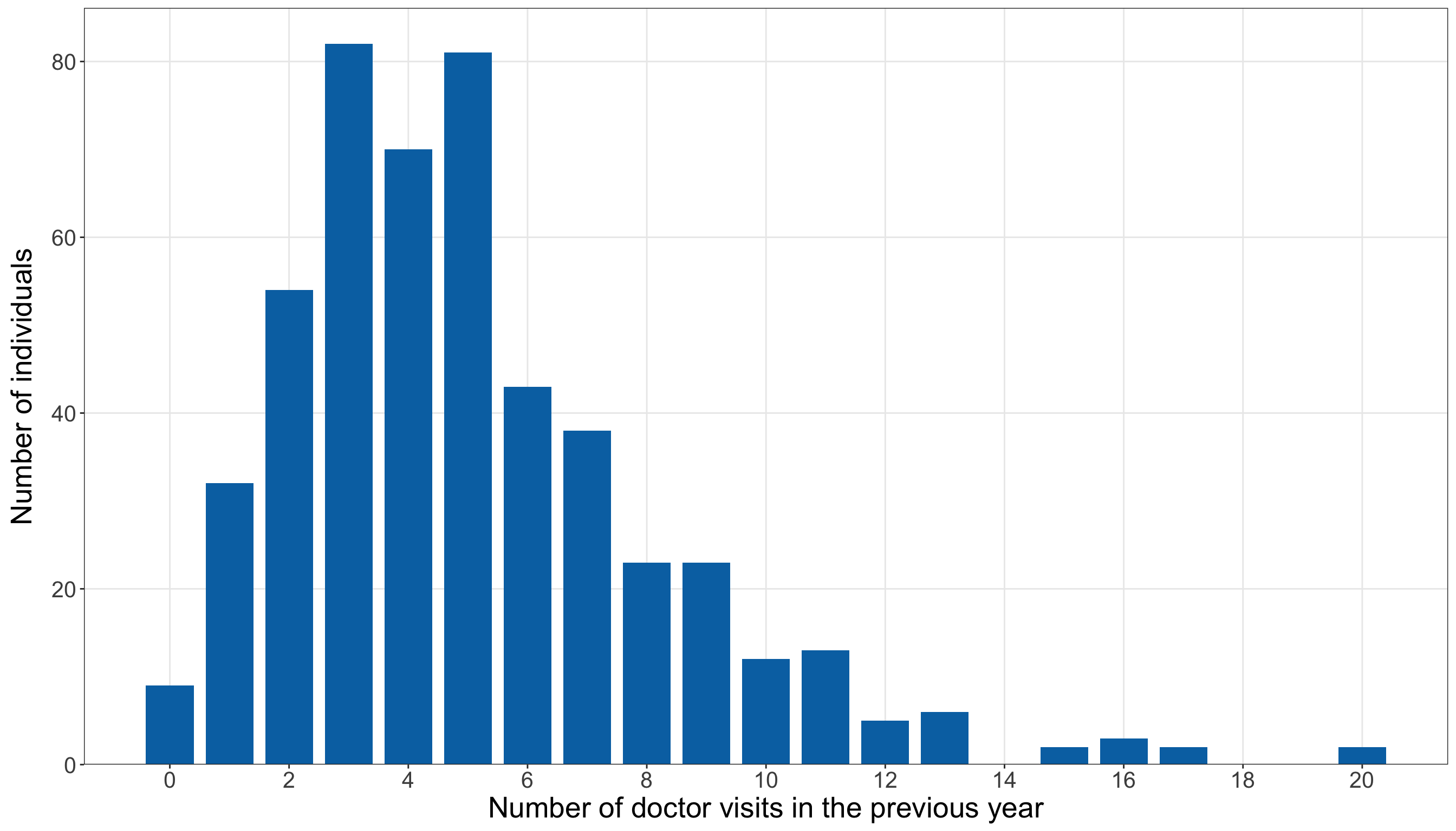
import matplotlib.pyplot as plt

doctor_response_frequencies = (
    doctor_training_data["doctor_visits"]
    .value_counts()
    .sort_index()
    .reindex(
        range(
            int(doctor_training_data["doctor_visits"].min()),
            int(doctor_training_data["doctor_visits"].max()) + 1,
        ),
        fill_value=0,
    )
)

(
    doctor_response_distribution_figure,
    doctor_response_distribution_axis,
) = plt.subplots(
    figsize=(14, 8)
)

_ = doctor_response_distribution_axis.bar(
    doctor_response_frequencies.index,
    doctor_response_frequencies.values,
    width=0.8,
    color="#0072B2",
)

_ = doctor_response_distribution_axis.set_xlabel(
    "Number of doctor visits in the previous year",
    fontsize=20,
)

_ = doctor_response_distribution_axis.set_ylabel(
    "Number of individuals",
    fontsize=20,
    labelpad=12,
)

_ = doctor_response_distribution_axis.set_xticks(
    range(
        0,
        int(doctor_response_frequencies.index.max()) + 1,
        2,
    )
)

doctor_response_distribution_axis.tick_params(
    axis="both",
    labelsize=15.5,
)

doctor_response_distribution_axis.grid(
    True,
    which="major",
    axis="both",
    alpha=0.3,
)

doctor_response_distribution_axis.grid(
    False,
    which="minor",
)

doctor_response_distribution_figure.tight_layout()
plt.show()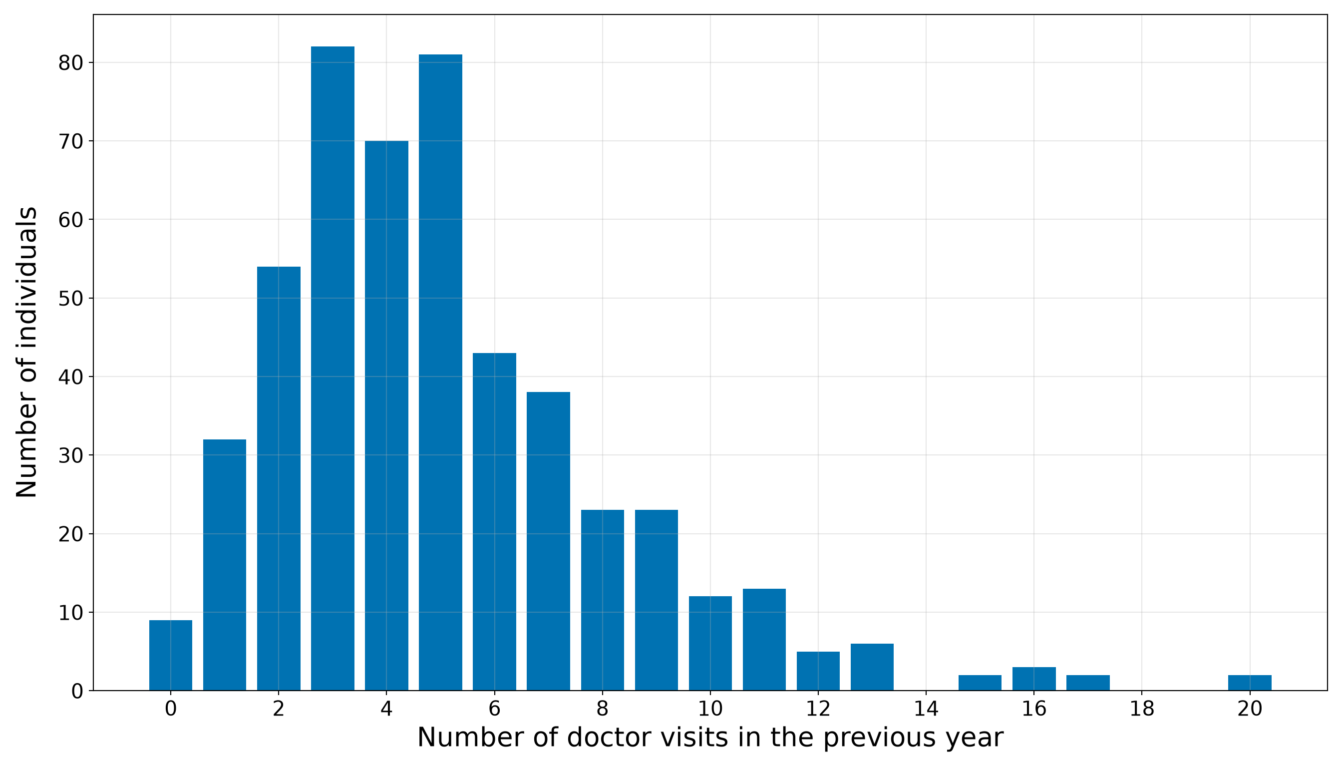
Figure 10.20 (or Figure 10.21) shows that the counts are concentrated mostly between approximately three and seven visits, with a thinner right tail extending to 20 visits. The horizontal support is entirely discrete and non-negative, so Poisson regression remains a natural starting model.
The variance-to-mean ratio above one is an exploratory warning, not a verdict against the model. The comparison in Table 10.88 is marginal: it ignores age, income, education, marriage status, residence, and insurance. Classical Poisson regression concerns the variance conditional on the regressors. Consequently, we will revisit the mean-variance relationship through fitted-model diagnostics after specifying and estimating the regression model.
Question 10.33 — Exploring the Continuous Regressors
Using only the training data:
- Divide
age,income, andeducation_yearsseparately into four equally sized groups based on their observed ordering. - Within each regressor quartile, report the number of individuals, mean regressor value, mean and median number of doctor visits, and proportion with zero visits.
- Construct scatterplots of
doctor_visitsagainst each continuous regressor and add a LOWESS/LOESS curve as a visual guide. - Describe the unadjusted patterns and identify one continuous regressor that provides a clear starting point for the simple Poisson regression model.
Answer 10.33
Click here to reveal the answer!
We first summarize the response across quartiles of each continuous regressor. Creating quartiles is only a descriptive device: it makes broad patterns easier to compare without claiming that the regressors are intrinsically categorical or that the relationship must change abruptly at the quartile boundaries.
doctor_continuous_long <- doctor_training_data |>
  select(
    doctor_visits,
    age,
    income,
    education_years
  ) |>
  pivot_longer(
    cols = c(
      age,
      income,
      education_years
    ),
    names_to = "regressor",
    values_to = "regressor_value"
  ) |>
  group_by(regressor) |>
  mutate(
    quartile_number = ntile(
      regressor_value,
      4
    )
  ) |>
  ungroup()

doctor_continuous_quartile_summary <- doctor_continuous_long |>
  group_by(
    regressor,
    quartile_number
  ) |>
  summarize(
    number_of_individuals = n(),
    mean_regressor_value = mean(regressor_value),
    mean_doctor_visits = mean(doctor_visits),
    median_doctor_visits = median(doctor_visits),
    proportion_zero_visits = mean(doctor_visits == 0),
    .groups = "drop"
  ) |>
  mutate(
    regressor_order = match(
      regressor,
      c(
        "age",
        "income",
        "education_years"
      )
    )
  ) |>
  arrange(
    regressor_order,
    quartile_number
  ) |>
  select(-regressor_order)

doctor_continuous_quartile_summary_display <-
  doctor_continuous_quartile_summary |>
  mutate(
    regressor = recode(
      regressor,
      age = "Age",
      income = "Income",
      education_years = "Education"
    ),
    quartile = paste0(
      "Q",
      quartile_number
    ),
    mean_regressor_value = case_when(
      regressor == "Income" ~ formatC(
        mean_regressor_value,
        format = "f",
        digits = 2,
        big.mark = ","
      ),
      TRUE ~ formatC(
        mean_regressor_value,
        format = "f",
        digits = 2
      )
    ),
    mean_doctor_visits = formatC(
      mean_doctor_visits,
      format = "f",
      digits = 3
    ),
    median_doctor_visits = formatC(
      median_doctor_visits,
      format = "f",
      digits = 1
    ),
    proportion_zero_visits = formatC(
      proportion_zero_visits,
      format = "f",
      digits = 3
    )
  ) |>
  select(
    regressor,
    quartile,
    number_of_individuals,
    mean_regressor_value,
    mean_doctor_visits,
    median_doctor_visits,
    proportion_zero_visits
  )

doctor_continuous_quartile_summary_display |>
  rename(
    `Regressor` = regressor,
    `Quartile` = quartile,
    `Number of individuals` = number_of_individuals,
    `Mean regressor value` = mean_regressor_value,
    `Mean doctor visits` = mean_doctor_visits,
    `Median doctor visits` = median_doctor_visits,
    `Proportion with zero visits` = proportion_zero_visits
  ) |>
  kable(
    align = rep("c", 7)
)| Regressor | Quartile | Number of individuals | Mean regressor value | Mean doctor visits | Median doctor visits | Proportion with zero visits |
|---|---|---|---|---|---|---|
| Age | Q1 | 125 | 21.33 | 3.400 | 3.0 | 0.040 |
| Age | Q2 | 125 | 31.45 | 4.320 | 4.0 | 0.016 |
| Age | Q3 | 125 | 37.48 | 5.160 | 5.0 | 0.008 |
| Age | Q4 | 125 | 47.03 | 7.432 | 7.0 | 0.008 |
| Income | Q1 | 125 | 30,963.58 | 6.496 | 6.0 | 0.000 |
| Income | Q2 | 125 | 46,427.67 | 4.936 | 4.0 | 0.008 |
| Income | Q3 | 125 | 55,961.28 | 4.864 | 4.0 | 0.032 |
| Income | Q4 | 125 | 69,055.10 | 4.016 | 4.0 | 0.032 |
| Education | Q1 | 125 | 10.98 | 4.032 | 4.0 | 0.024 |
| Education | Q2 | 125 | 13.77 | 4.800 | 4.0 | 0.048 |
| Education | Q3 | 125 | 16.25 | 5.376 | 5.0 | 0.000 |
| Education | Q4 | 125 | 19.05 | 6.104 | 5.0 | 0.000 |
doctor_continuous_regressors = {
    "age": "Age",
    "income": "Income",
    "education_years": "Education",
}

doctor_continuous_quartile_tables = []

for regressor, regressor_label in (
    doctor_continuous_regressors.items()
):
    regressor_data = doctor_training_data[
        [regressor, "doctor_visits"]
    ].copy()

    # The first-occurrence rank reproduces R's handling of ties in ntile().
    regressor_data["Quartile"] = pd.qcut(
        regressor_data[regressor].rank(
            method="first"
        ),
        q=4,
        labels=[
            "Q1",
            "Q2",
            "Q3",
            "Q4",
        ],
    )

    regressor_summary = (
        regressor_data
        .groupby(
            "Quartile",
            observed=False,
        )
        .agg(
            Number_of_individuals=(
                "doctor_visits",
                "size",
            ),
            Mean_regressor_value=(
                regressor,
                "mean",
            ),
            Mean_doctor_visits=(
                "doctor_visits",
                "mean",
            ),
            Median_doctor_visits=(
                "doctor_visits",
                "median",
            ),
            Proportion_zero_visits=(
                "doctor_visits",
                lambda values: (
                    values == 0
                ).mean(),
            ),
        )
        .reset_index()
    )

    regressor_summary.insert(
        0,
        "Regressor",
        regressor_label,
    )

    doctor_continuous_quartile_tables.append(
        regressor_summary
    )

doctor_continuous_quartile_summary = pd.concat(
    doctor_continuous_quartile_tables,
    ignore_index=True,
)

doctor_continuous_quartile_summary_display = (
    doctor_continuous_quartile_summary.copy()
)

doctor_continuous_quartile_summary_display[
    "Mean regressor value"
] = doctor_continuous_quartile_summary_display.apply(
    lambda row: (
        f"{row['Mean_regressor_value']:,.2f}"
        if row["Regressor"] == "Income"
        else f"{row['Mean_regressor_value']:.2f}"
    ),
    axis=1,
)

doctor_continuous_quartile_summary_display[
    "Mean doctor visits"
] = doctor_continuous_quartile_summary_display[
    "Mean_doctor_visits"
].map(lambda value: f"{value:.3f}")

doctor_continuous_quartile_summary_display[
    "Median doctor visits"
] = doctor_continuous_quartile_summary_display[
    "Median_doctor_visits"
].map(lambda value: f"{value:.1f}")

doctor_continuous_quartile_summary_display[
    "Proportion with zero visits"
] = doctor_continuous_quartile_summary_display[
    "Proportion_zero_visits"
].map(lambda value: f"{value:.3f}")

doctor_continuous_quartile_summary_display = (
    doctor_continuous_quartile_summary_display
    .rename(
        columns={
            "Number_of_individuals": (
                "Number of individuals"
            ),
        }
    )
    [
        [
            "Regressor",
            "Quartile",
            "Number of individuals",
            "Mean regressor value",
            "Mean doctor visits",
            "Median doctor visits",
            "Proportion with zero visits",
        ]
    ]
)

doctor_continuous_quartile_summary_html = (
    doctor_continuous_quartile_summary_display.to_html(
        index=False,
        border=0,
    )
)| Regressor | Quartile | Number of individuals | Mean regressor value | Mean doctor visits | Median doctor visits | Proportion with zero visits |
|---|---|---|---|---|---|---|
| Age | Q1 | 125 | 21.33 | 3.400 | 3.0 | 0.040 |
| Age | Q2 | 125 | 31.45 | 4.320 | 4.0 | 0.016 |
| Age | Q3 | 125 | 37.48 | 5.160 | 5.0 | 0.008 |
| Age | Q4 | 125 | 47.03 | 7.432 | 7.0 | 0.008 |
| Income | Q1 | 125 | 30,963.58 | 6.496 | 6.0 | 0.000 |
| Income | Q2 | 125 | 46,427.67 | 4.936 | 4.0 | 0.008 |
| Income | Q3 | 125 | 55,961.28 | 4.864 | 4.0 | 0.032 |
| Income | Q4 | 125 | 69,055.10 | 4.016 | 4.0 | 0.032 |
| Education | Q1 | 125 | 10.98 | 4.032 | 4.0 | 0.024 |
| Education | Q2 | 125 | 13.77 | 4.800 | 4.0 | 0.048 |
| Education | Q3 | 125 | 16.25 | 5.376 | 5.0 | 0.000 |
| Education | Q4 | 125 | 19.05 | 6.104 | 5.0 | 0.000 |
The quartile summaries in Table 10.90 reveal three distinct unadjusted patterns:
- Age: The mean number of doctor visits rises from 3.400 in the youngest quartile to 7.432 in the oldest quartile. The corresponding mean ages are 21.33 and 47.03 years.
- Income: The mean count decreases from 6.496 in the lowest-income quartile to 4.016 in the highest-income quartile.
- Education: The mean count increases from 4.032 in the lowest-education quartile to 6.104 in the highest-education quartile.
These summaries do not adjust for the remaining characteristics. In particular, they do not establish that changing age, income, or education would cause a change in health-care use. They show only how annual doctor-visit counts vary descriptively across the observed training sample.
Now, we return the continuous regressors to their original scales. In the plots below, the blue points show the observed count-regressor pairs. The orange LOWESS/LOESS curves are flexible visual guides fitted locally through the point clouds. They are not Poisson regression fits, and we use them only to inspect direction and possible curvature before specifying the regression models.
doctor_continuous_plot_data <- doctor_continuous_long |>
  mutate(
    regressor = factor(
      regressor,
      levels = c(
        "age",
        "income",
        "education_years"
      ),
      labels = c(
        "Age (years)",
        "Income (dollars)",
        "Education (years)"
      )
    )
  )

doctor_continuous_patterns_plot <- ggplot(
  doctor_continuous_plot_data,
  aes(
    x = regressor_value,
    y = doctor_visits
  )
) +
  geom_point(
    colour = "#0072B2",
    alpha = 0.35,
    size = 1.8
  ) +
  geom_smooth(
    method = "loess",
    formula = y ~ x,
    span = 0.75,
    se = FALSE,
    colour = "#D55E00",
    linewidth = 1.2
  ) +
  facet_wrap(
    ~regressor,
    scales = "free_x",
    nrow = 1
  ) +
  scale_y_continuous(
    breaks = seq(
      0,
      max(doctor_training_data$doctor_visits),
      by = 2
    )
  ) +
  theme_bw() +
  theme(
    axis.text = element_text(size = 15.5),
    axis.title.x = element_text(size = 20),
    axis.title.y = element_text(
      size = 20,
      vjust = 0.5,
      margin = margin(r = 12)
    ),
    strip.text = element_text(
      size = 20,
      face = "bold"
    ),
    panel.grid.minor = element_blank()
  ) +
  labs(
    x = "Regressor value",
    y = "Number of doctor visits"
  )

doctor_continuous_patterns_plot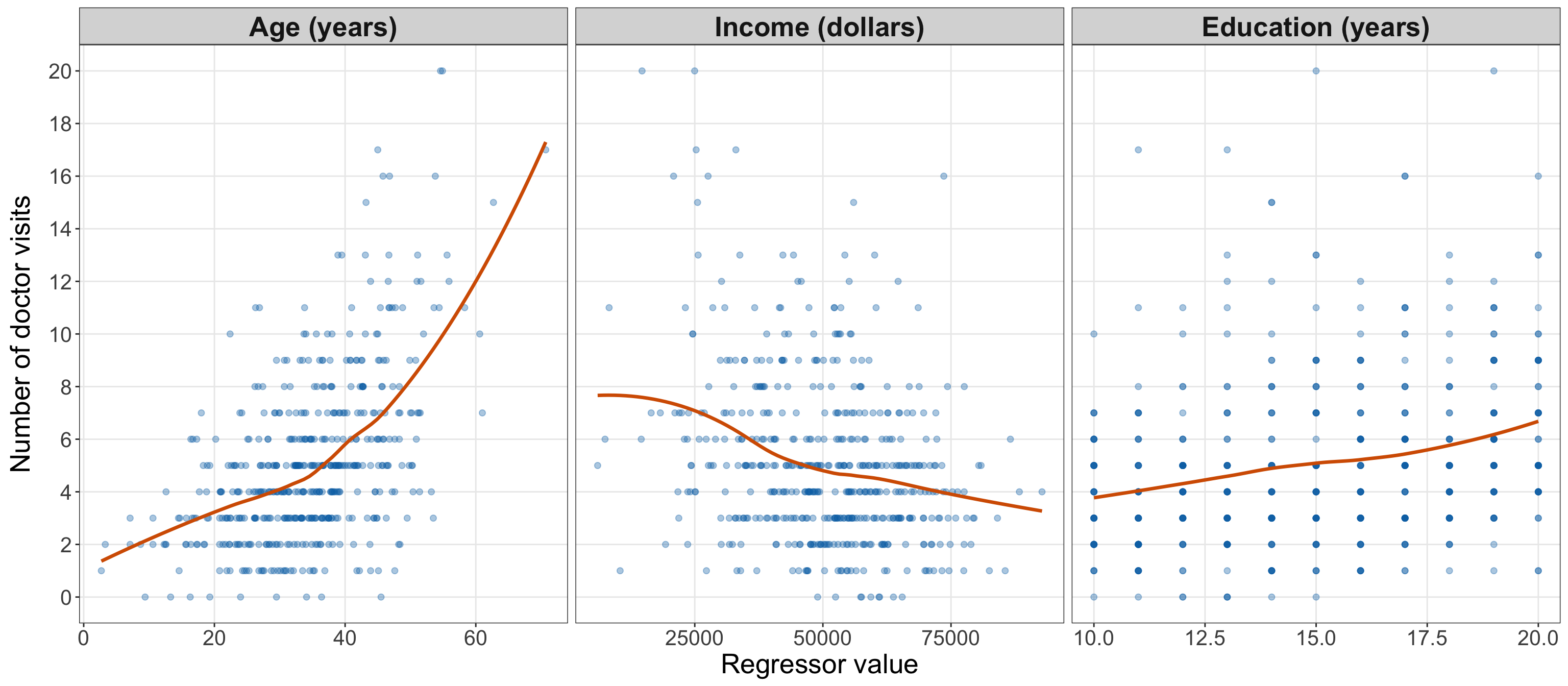
from statsmodels.nonparametric.smoothers_lowess import lowess

doctor_continuous_plot_specifications = [
    (
        "age",
        "Age (years)",
    ),
    (
        "income",
        "Income (dollars)",
    ),
    (
        "education_years",
        "Education (years)",
    ),
]

(
    doctor_continuous_patterns_figure,
    doctor_continuous_patterns_axes,
) = plt.subplots(
    1,
    3,
    figsize=(16, 7),
    sharey=True,
)

for axis, (regressor, axis_label) in zip(
    doctor_continuous_patterns_axes,
    doctor_continuous_plot_specifications,
):
    x_values = doctor_training_data[
        regressor
    ].to_numpy()

    y_values = doctor_training_data[
        "doctor_visits"
    ].to_numpy()

    smooth_values = lowess(
        y_values,
        x_values,
        frac=0.75,
        it=0,
        return_sorted=True,
    )

    _ = axis.scatter(
        x_values,
        y_values,
        alpha=0.35,
        s=22,
        color="#0072B2",
    )

    _ = axis.plot(
        smooth_values[:, 0],
        smooth_values[:, 1],
        linewidth=2.2,
        color="#D55E00",
    )

    _ = axis.set_title(
        axis_label,
        fontsize=20,
        fontweight="bold",
    )

    _ = axis.set_xlabel(
        "Regressor value",
        fontsize=20,
    )

    axis.tick_params(
        axis="both",
        labelsize=15.5,
    )

    axis.grid(
        True,
        which="major",
        axis="both",
        alpha=0.3,
    )

    axis.grid(
        False,
        which="minor",
    )

_ = doctor_continuous_patterns_axes[0].set_ylabel(
    "Number of doctor visits",
    fontsize=20,
    labelpad=12,
)

_ = doctor_continuous_patterns_axes[0].set_yticks(
    range(
        0,
        int(doctor_training_data["doctor_visits"].max()) + 1,
        2,
    )
)

doctor_continuous_patterns_figure.tight_layout()
plt.show()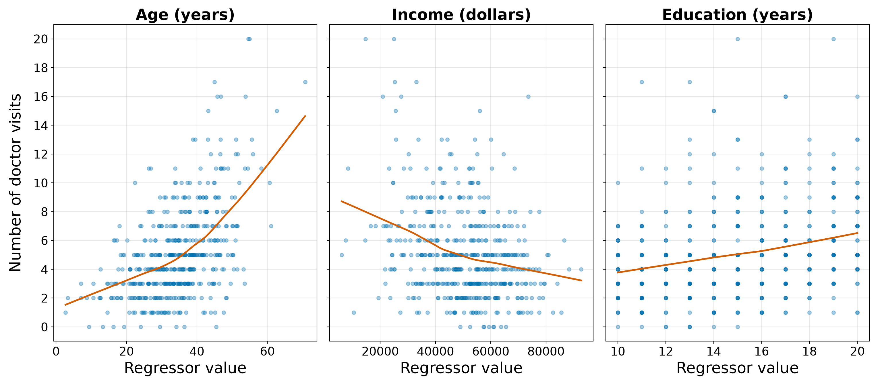
The plots in Figure 10.22 (or Figure 10.23) reinforce the quartile summaries. Doctor visits show a clear increasing pattern with age, a decreasing pattern with income, and a more moderate increasing pattern with years of education. There is also substantial vertical spread around each curve: individuals with similar regressor values can report noticeably different annual counts.
Among the three continuous regressors, age provides the clearest starting point for the simple model. Its quartile means increase consistently, and its exploratory smooth shows a pronounced positive association. We will therefore begin with an age-only Poisson regression before considering the remaining demographic and socioeconomic characteristics in the extended model. This choice is a modelling starting point motivated by the training EDA, not a final inferential conclusion.
Question 10.34 — Exploring the Categorical Regressors
Using only the training data:
- For each category of
married,urban, andinsurance, report the number of individuals, mean and median number of doctor visits, and proportion with zero visits. - Construct boxplots with horizontally jittered observations to compare the count distributions across categories.
- Describe the unadjusted differences while accounting for category overlap and the observational nature of the data.
Answer 10.34
Click here to reveal the answer!
The following summaries compare the annual count distribution within each observed category. The sample sizes are reported alongside the response summaries so that apparent differences are not interpreted without considering how many individuals support each comparison.
doctor_categorical_long <- doctor_training_data |>
  mutate(
    across(
      c(
        married,
        urban,
        insurance
      ),
      as.character
    )
  ) |>
  select(
    doctor_visits,
    married,
    urban,
    insurance
  ) |>
  pivot_longer(
    cols = c(
      married,
      urban,
      insurance
    ),
    names_to = "regressor",
    values_to = "category"
  ) |>
  mutate(
    regressor = factor(
      regressor,
      levels = c(
        "married",
        "urban",
        "insurance"
      )
    ),
    category = factor(
      category,
      levels = c(
        "Not married",
        "Married",
        "Non-urban",
        "Urban",
        "Uninsured",
        "Insured"
      )
    )
  )

doctor_categorical_summary <- doctor_categorical_long |>
  group_by(
    regressor,
    category,
  ) |>
  summarize(
    number_of_individuals = n(),
    mean_doctor_visits = mean(doctor_visits),
    median_doctor_visits = median(doctor_visits),
    proportion_zero_visits = mean(doctor_visits == 0),
    .groups = "drop"
  ) |>
  filter(number_of_individuals > 0) |>
  arrange(
    regressor,
    category
  )

doctor_categorical_summary_display <- doctor_categorical_summary |>
  mutate(
    regressor = recode(
      as.character(regressor),
      married = "Marriage status",
      urban = "Residence",
      insurance = "Insurance status"
    ),
    mean_doctor_visits = formatC(
      mean_doctor_visits,
      format = "f",
      digits = 3
    ),
    median_doctor_visits = formatC(
      median_doctor_visits,
      format = "f",
      digits = 1
    ),
    proportion_zero_visits = formatC(
      proportion_zero_visits,
      format = "f",
      digits = 3
    )
  )

doctor_categorical_summary_display |>
  rename(
    `Regressor` = regressor,
    `Category` = category,
    `Number of individuals` = number_of_individuals,
    `Mean doctor visits` = mean_doctor_visits,
    `Median doctor visits` = median_doctor_visits,
    `Proportion with zero visits` = proportion_zero_visits
  ) |>
  kable(
    align = rep("c", 6)
)| Regressor | Category | Number of individuals | Mean doctor visits | Median doctor visits | Proportion with zero visits |
|---|---|---|---|---|---|
| Marriage status | Not married | 249 | 4.815 | 4.0 | 0.028 |
| Marriage status | Married | 251 | 5.339 | 5.0 | 0.008 |
| Residence | Non-urban | 148 | 4.588 | 4.0 | 0.007 |
| Residence | Urban | 352 | 5.284 | 5.0 | 0.023 |
| Insurance status | Uninsured | 197 | 4.487 | 4.0 | 0.030 |
| Insurance status | Insured | 303 | 5.462 | 5.0 | 0.010 |
doctor_categorical_specifications = {
    "married": {
        "label": "Marriage status",
        "categories": [
            "Not married",
            "Married",
        ],
    },
    "urban": {
        "label": "Residence",
        "categories": [
            "Non-urban",
            "Urban",
        ],
    },
    "insurance": {
        "label": "Insurance status",
        "categories": [
            "Uninsured",
            "Insured",
        ],
    },
}

doctor_categorical_summary_tables = []

for regressor, specification in (
    doctor_categorical_specifications.items()
):
    category_summary = (
        doctor_training_data
        .groupby(
            regressor,
            observed=False,
        )
        .agg(
            Number_of_individuals=(
                "doctor_visits",
                "size",
            ),
            Mean_doctor_visits=(
                "doctor_visits",
                "mean",
            ),
            Median_doctor_visits=(
                "doctor_visits",
                "median",
            ),
            Proportion_zero_visits=(
                "doctor_visits",
                lambda values: (
                    values == 0
                ).mean(),
            ),
        )
        .reindex(
            specification["categories"]
        )
        .reset_index()
        .rename(
            columns={
                regressor: "Category",
            }
        )
    )

    category_summary.insert(
        0,
        "Regressor",
        specification["label"],
    )

    doctor_categorical_summary_tables.append(
        category_summary
    )

doctor_categorical_summary = pd.concat(
    doctor_categorical_summary_tables,
    ignore_index=True,
)

doctor_categorical_summary_display = (
    doctor_categorical_summary
    .rename(
        columns={
            "Number_of_individuals": (
                "Number of individuals"
            ),
        }
    )
    .copy()
)

doctor_categorical_summary_display[
    "Mean doctor visits"
] = doctor_categorical_summary_display[
    "Mean_doctor_visits"
].map(lambda value: f"{value:.3f}")

doctor_categorical_summary_display[
    "Median doctor visits"
] = doctor_categorical_summary_display[
    "Median_doctor_visits"
].map(lambda value: f"{value:.1f}")

doctor_categorical_summary_display[
    "Proportion with zero visits"
] = doctor_categorical_summary_display[
    "Proportion_zero_visits"
].map(lambda value: f"{value:.3f}")

doctor_categorical_summary_display = (
    doctor_categorical_summary_display[
        [
            "Regressor",
            "Category",
            "Number of individuals",
            "Mean doctor visits",
            "Median doctor visits",
            "Proportion with zero visits",
        ]
    ]
)

classical_poisson_exercise_doctor_categorical_summary_py_html = (
    doctor_categorical_summary_display.to_html(
        index=False,
        border=0,
    )
)| Regressor | Category | Number of individuals | Mean doctor visits | Median doctor visits | Proportion with zero visits |
|---|---|---|---|---|---|
| Marriage status | Not married | 249 | 4.815 | 4.0 | 0.028 |
| Marriage status | Married | 251 | 5.339 | 5.0 | 0.008 |
| Residence | Non-urban | 148 | 4.588 | 4.0 | 0.007 |
| Residence | Urban | 352 | 5.284 | 5.0 | 0.023 |
| Insurance status | Uninsured | 197 | 4.487 | 4.0 | 0.030 |
| Insurance status | Insured | 303 | 5.462 | 5.0 | 0.010 |
The training-set comparisons in Table 10.92 show the following:
- Marriage status: The 249 not-married individuals report a mean of 4.815 visits, compared with 5.339 among the 251 married individuals.
- Residence: The mean is 4.588 visits among non-urban residents and 5.284 among urban residents.
- Insurance status: Uninsured individuals report a mean of 4.487 visits, while insured individuals report a mean of 5.462.
The largest unadjusted mean difference among these three binary comparisons appears for insurance status, followed by residence. Nevertheless, these are not like-for-like adjusted comparisons. For example, insured and uninsured individuals may differ in age, income, education, or residence. The extended Poisson regression will later examine these regressors jointly.
The table summarizes centres and zero proportions, but it does not show how much the count distributions overlap. The following boxplots and points supply that information. Horizontal jitter separates observations that would otherwise appear at the same category position; it does not alter the observed counts on the vertical axis.
set.seed(123)

doctor_categorical_plot_data <- doctor_categorical_long |>
  mutate(
    regressor = factor(
      regressor,
      levels = c(
        "married",
        "urban",
        "insurance"
      ),
      labels = c(
        "Marriage status",
        "Residence",
        "Insurance status"
      )
    )
  )

doctor_categorical_comparisons_plot <- ggplot(
  doctor_categorical_plot_data,
  aes(
    x = category,
    y = doctor_visits
  )
) +
  geom_boxplot(
    fill = "#0072B2",
    alpha = 0.45,
    outlier.shape = NA
  ) +
  geom_point(
    position = position_jitter(
      width = 0.18,
      height = 0,
      seed = 123
    ),
    colour = "#D55E00",
    alpha = 0.45,
    size = 1.6
  ) +
  facet_wrap(
    ~regressor,
    scales = "free_x",
    nrow = 1
  ) +
  scale_y_continuous(
    breaks = seq(
      0,
      max(doctor_training_data$doctor_visits),
      by = 2
    )
  ) +
  theme_bw() +
  theme(
    axis.text = element_text(size = 15.5),
    axis.title.x = element_text(size = 20),
    axis.title.y = element_text(
      size = 20,
      vjust = 0.5,
      margin = margin(r = 12)
    ),
    strip.text = element_text(
      size = 20,
      face = "bold"
    ),
    panel.grid.minor = element_blank()
  ) +
  labs(
    x = "Category",
    y = "Number of doctor visits"
  )

doctor_categorical_comparisons_plot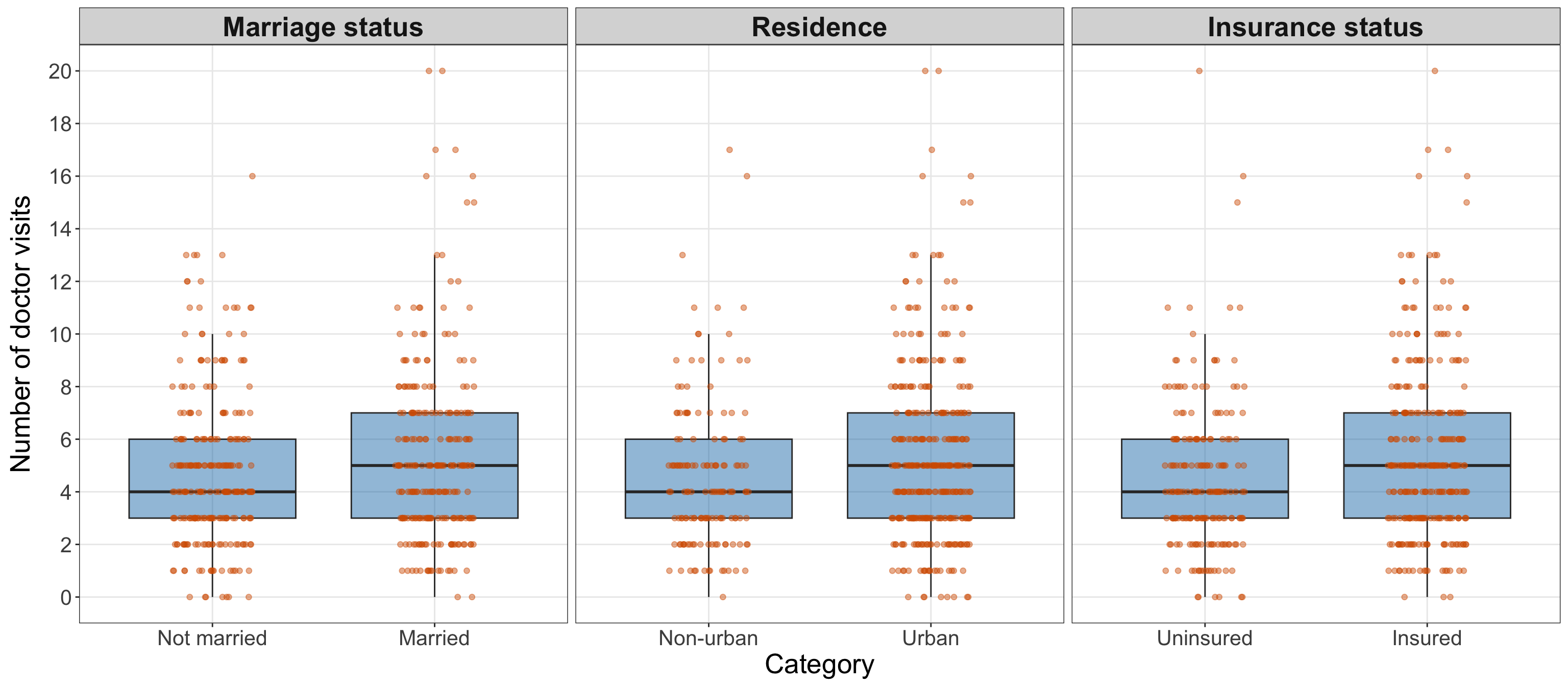
doctor_categorical_plot_specifications = [
    (
        "married",
        "Marriage status",
        [
            "Not married",
            "Married",
        ],
    ),
    (
        "urban",
        "Residence",
        [
            "Non-urban",
            "Urban",
        ],
    ),
    (
        "insurance",
        "Insurance status",
        [
            "Uninsured",
            "Insured",
        ],
    ),
]

doctor_categorical_rng = np.random.default_rng(
    123
)

(
    doctor_categorical_comparisons_figure,
    doctor_categorical_comparisons_axes,
) = plt.subplots(
    1,
    3,
    figsize=(16, 7),
    sharey=True,
)

for axis, (
    regressor,
    axis_title,
    categories,
) in zip(
    doctor_categorical_comparisons_axes,
    doctor_categorical_plot_specifications,
):
    category_values = [
        doctor_training_data.loc[
            doctor_training_data[regressor] == category,
            "doctor_visits",
        ].to_numpy()
        for category in categories
    ]

    category_boxplots = axis.boxplot(
        category_values,
        tick_labels=categories,
        patch_artist=True,
        showfliers=False,
    )

    for patch in category_boxplots["boxes"]:
        patch.set_facecolor("#0072B2")
        patch.set_alpha(0.45)

    for category_position, values in enumerate(
        category_values,
        start=1,
    ):
        jittered_positions = (
            category_position
            + doctor_categorical_rng.uniform(
                -0.18,
                0.18,
                size=len(values),
            )
        )

        _ = axis.scatter(
            jittered_positions,
            values,
            color="#D55E00",
            alpha=0.45,
            s=22,
        )

    _ = axis.set_title(
        axis_title,
        fontsize=20,
        fontweight="bold",
    )

    _ = axis.set_xlabel(
        "Category",
        fontsize=20,
    )

    axis.tick_params(
        axis="both",
        labelsize=15.5,
    )

    axis.grid(
        True,
        which="major",
        axis="both",
        alpha=0.3,
    )

    axis.grid(
        False,
        which="minor",
    )

_ = doctor_categorical_comparisons_axes[0].set_ylabel(
    "Number of doctor visits",
    fontsize=20,
    labelpad=12,
)

_ = doctor_categorical_comparisons_axes[0].set_yticks(
    range(
        0,
        int(doctor_training_data["doctor_visits"].max()) + 1,
        2,
    )
)

doctor_categorical_comparisons_figure.tight_layout()
plt.show()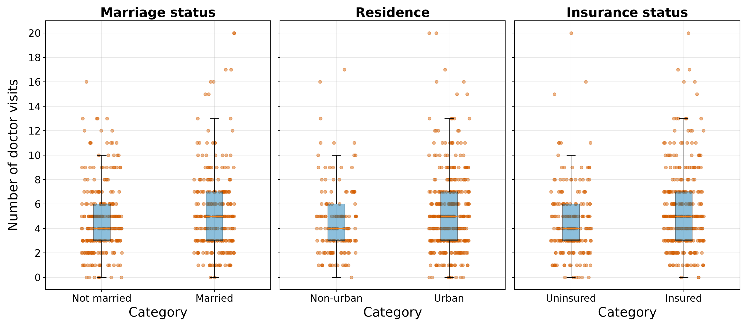
Figure 10.24 (or Figure 10.25) show substantial overlap within every pair of categories. Higher and lower counts occur in each marriage, residence, and insurance group. The differences in group means may therefore be useful for the extended model, but none of the categorical regressors separates annual doctor visits cleanly on its own.
These comparisons remain descriptive. They do not establish that marriage, urban residence, or insurance coverage causes a change in the number of doctor visits. Formal coefficient interpretation must wait until the regressors are included jointly in the Poisson regression model.
Question 10.35 — Translating the EDA into Modelling Decisions
Summarize the main findings from the training-set EDA. Explain:
- why Classical Poisson regression remains a reasonable starting model;
- which feature of the response requires careful later checking;
- which regressor will be used in the simple model; and
- why the remaining regressors should still be considered in an extended model.
Answer 10.35
Click here to reveal the answer!
Table 10.94 condenses the EDA findings and connects them to the next stages of the workflow.
| EDA component | Main training-set finding | Consequence for the modelling workflow |
|---|---|---|
| Data split | The common R-generated split contains 500 training observations and 500 testing observations. |
All exploration and model development will use the training set. The testing set remains untouched until the final predictive assessment and inferential refit. |
| Count response |
doctor_visits is a non-negative integer count ranging from 0 to 20. The mean is 5.078 and the sample variance is 10.192. |
Poisson regression is a natural starting point, but the variance-to-mean ratio of 2.007 motivates careful goodness-of-fit and equidispersion checks after fitting. |
| Continuous regressors | Doctor visits increase clearly across age quartiles, decrease across income quartiles, and increase more moderately across education quartiles. | Age supplies a transparent regressor for the simple model. Income and education remain candidates for the extended model because they show additional descriptive structure. |
| Categorical regressors | Married, urban, and insured individuals have higher unadjusted mean counts than their respective baseline groups, but the category distributions overlap substantially. | Marriage status, residence, and insurance should be considered jointly with the continuous regressors rather than interpreted from isolated group comparisons. |
| Scope of interpretation | Every pattern comes from observational training data and is unadjusted unless explicitly stated otherwise. | The EDA motivates model specification; it does not establish causality, statistical significance, model adequacy, or out-of-sample predictive performance. |
The next modelling step will therefore use age in a simple Poisson regression. This first model will let us introduce estimation and expected-count interpretation with one clearly motivated regressor. We will then fit an extended model containing age, income, years of education, marriage status, residence, and insurance status. The extended model is necessary because the descriptive patterns can overlap: a marginal difference associated with one regressor may change after the remaining characteristics are held fixed.
Finally, the unconditional variance exceeding the unconditional mean does not by itself reject the Classical Poisson model. The decisive checks concern the fitted conditional model. We will assess those checks after estimating the simple and extended Poisson regressions, before using either model for the case study’s inferential and predictive conclusions.
Simple Classical Poisson Regression and Goodness of Fit
The EDA identified age as the clearest continuous starting point for a simple model. We now use the training data to estimate an age-only Classical Poisson regression and then ask whether that model adequately reproduces important features of the observed counts. This is still part of model development: the testing data remain untouched, and the coefficient estimates below are not used for the final inferential conclusions.
Question 10.36 — Specifying and Fitting the Simple Age-Only Poisson Regression
Using doctor_training_data:
- Let \(Y_i\) denote the annual number of doctor visits for the \(i\)th individual and let \(x_{i,1}\) denote that individual’s age in years. Write the random component, systematic component, and log-link formulation of a simple Classical Poisson regression.
- Fit the model in
RandPythonusing onlyageas a regressor. - Report the maximum likelihood estimates, model-based standard errors, exponentiated estimates, and corresponding percentage changes.
- Interpret the fitted age coefficient as a training-set association, both for a one-year increase and for a ten-year increase in age.
- Compute the fitted expected number of doctor visits for individuals aged 20, 40, and 60 years.
- Explain why these training-set estimates should not yet be treated as the final inferential results for the case study.
Answer 10.36
Click here to reveal the answer!
For the \(i\)th individual in the training data, let
\[ Y_i = \text{annual number of doctor visits} \]
and
\[ x_{i,1} = \text{age in years}. \]
The simple Classical Poisson regression is
\[ Y_i \mid x_{i,1} \sim \operatorname{Poisson}(\mu_i), \]
with systematic component and log link
\[ \log(\mu_i) = \beta_0 + \beta_1 x_{i,1}. \]
Equivalently, the conditional expected count is
\[ \mu_i = \exp(\beta_0 + \beta_1 x_{i,1}). \tag{10.22}\]
Under the Classical Poisson assumption,
\[ \mathbb{E}(Y_i \mid x_{i,1}) = \operatorname{Var}(Y_i \mid x_{i,1}) = \mu_i. \]
Thus, age determines the fitted conditional mean through Equation 10.22, while the random component imposes the corresponding conditional equidispersion assumption.
Now, we fit the model on the training set:
- In
R,glm()usesfamily = poisson(link = "log"). - In
Python, the analogous model is fitted withsmf.glm()andsm.families.Poisson().
The table below includes the exponentiated estimate because \(\exp(\hat\beta_1)\) is the fitted multiplicative change in the expected count for a one-year increase in age.
library(broom)

# Fitting the age-only Classical Poisson regression
doctor_simple_poisson_model <- glm(
  formula = doctor_visits ~ age,
  family = poisson(link = "log"),
  data = doctor_training_data
)

# Retaining a numeric summary for later inline calculations
doctor_simple_poisson_summary <- tidy(
  doctor_simple_poisson_model
) |>
  mutate(
    exponentiated_estimate = exp(estimate),
    percent_change = 100 * (
      exponentiated_estimate - 1
    )
  )

# Quantities used in the interpretation
doctor_simple_age_estimate <- coef(
  doctor_simple_poisson_model
)[["age"]]

doctor_simple_age_multiplier <- exp(
  doctor_simple_age_estimate
)

doctor_simple_age_percent_change <- 100 * (
  doctor_simple_age_multiplier - 1
)

doctor_simple_age_decade_multiplier <- exp(
  10 * doctor_simple_age_estimate
)

doctor_simple_age_decade_percent_change <- 100 * (
  doctor_simple_age_decade_multiplier - 1
)

# Formatting only for display
doctor_simple_poisson_summary_display <-
  doctor_simple_poisson_summary |>
  mutate(
    across(
      c(
        estimate,
        std.error,
        exponentiated_estimate,
        percent_change
      ),
      ~ formatC(
        .x,
        format = "f",
        digits = 3
      )
    )
  )

doctor_simple_poisson_summary_display |>
  select(
    term,
    estimate,
    std.error,
    exponentiated_estimate,
    percent_change
  ) |>
  rename(
    `Term` = term,
    `Estimate` = estimate,
    `Standard error` = std.error,
    `Exponentiated estimate` = exponentiated_estimate,
    `Percent change` = percent_change
  ) |>
  kable(
    align = c("c", "c", "c", "c", "c")
)| Term | Estimate | Standard error | Exponentiated estimate | Percent change |
|---|---|---|---|---|
| (Intercept) | 0.444 | 0.077 | 1.559 | 55.945 |
| age | 0.033 | 0.002 | 1.033 | 3.335 |
import statsmodels.api as sm
import statsmodels.formula.api as smf

doctor_simple_poisson_model = smf.glm(
    formula="doctor_visits ~ age",
    data=doctor_training_data,
    family=sm.families.Poisson(),
).fit()

doctor_simple_poisson_summary = pd.DataFrame(
    {
        "Term": doctor_simple_poisson_model.params.index,
        "Estimate": doctor_simple_poisson_model.params.values,
        "Standard error": doctor_simple_poisson_model.bse.values,
        "Exponentiated estimate": np.exp(
            doctor_simple_poisson_model.params.values
        ),
    }
)

doctor_simple_poisson_summary["Percent change"] = 100 * (
    doctor_simple_poisson_summary[
        "Exponentiated estimate"
    ]
    - 1
)

doctor_simple_poisson_summary_display = (
    doctor_simple_poisson_summary.copy()
)

for column in [
    "Estimate",
    "Standard error",
    "Exponentiated estimate",
    "Percent change",
]:
    doctor_simple_poisson_summary_display[column] = (
        doctor_simple_poisson_summary_display[column]
        .map(lambda value: f"{value:.3f}")
    )

classical_poisson_exercise_doctor_simple_age_fit_py_html = (
    doctor_simple_poisson_summary_display.to_html(
        index=False,
        border=0,
    )
)| Term | Estimate | Standard error | Exponentiated estimate | Percent change |
|---|---|---|---|---|
| Intercept | 0.444 | 0.077 | 1.559 | 55.945 |
| age | 0.033 | 0.002 | 1.033 | 3.335 |
According to Table 10.95, the fitted age coefficient is 0.0328. Its positive sign indicates that the fitted expected number of doctor visits increases with age in the training data. More specifically, a one-year increase in age multiplies the fitted expected count by 1.0333, corresponding to an estimated 3.33% increase.
Because one year is a small unit on the age scale, a ten-year comparison can be easier to communicate. Holding the model structure fixed, a ten-year increase in age multiplies the fitted expected count by
\[ \exp(10\hat\beta_1), \]
which equals 1.388 for this fitted model. This corresponds to an estimated 38.8% increase in the expected annual count over a ten-year age difference.
The intercept is the fitted log expected count at age zero. Since age zero is outside the observed age range reported in Table 10.80, the intercept is needed mathematically but is not the main substantive quantity of interest.
To make the fitted relationship concrete on the response scale, we evaluate the model at ages 20, 40, and 60 years. The predictions use type = "response" in R; in Python, .predict() already returns fitted expected counts on the response scale for this model.
# Selected ages within the observed range
doctor_simple_age_predictions <- tibble(
  age = c(20, 40, 60)
)

doctor_simple_age_predictions <-
  doctor_simple_age_predictions |>
  mutate(
    fitted_expected_count = predict(
      doctor_simple_poisson_model,
      newdata = doctor_simple_age_predictions,
      type = "response"
    )
  )

doctor_simple_age_predictions |>
  mutate(
    fitted_expected_count = formatC(
      fitted_expected_count,
      format = "f",
      digits = 3
    )
  ) |>
  rename(
    `Age (years)` = age,
    `Fitted expected annual doctor visits` = fitted_expected_count
  ) |>
  kable(
    align = c("c", "c")
)| Age (years) | Fitted expected annual doctor visits |
|---|---|
| 20 | 3.005 |
| 40 | 5.792 |
| 60 | 11.164 |
# Selected ages within the observed range
doctor_simple_age_predictions = pd.DataFrame(
    {
        "Age (years)": [20, 40, 60],
    }
)

doctor_simple_age_predictions[
    "Fitted expected annual doctor visits"
] = doctor_simple_poisson_model.predict(
    pd.DataFrame(
        {
            "age": doctor_simple_age_predictions[
                "Age (years)"
            ]
        }
    )
)

doctor_simple_age_predictions_display = (
    doctor_simple_age_predictions.copy()
)

doctor_simple_age_predictions_display[
    "Fitted expected annual doctor visits"
] = doctor_simple_age_predictions_display[
    "Fitted expected annual doctor visits"
].map(lambda value: f"{value:.3f}")

classical_poisson_exercise_doctor_simple_age_predictions_py_html = (
    doctor_simple_age_predictions_display.to_html(
        index=False,
        border=0,
    )
)| Age (years) | Fitted expected annual doctor visits |
|---|---|
| 20 | 3.005 |
| 40 | 5.792 |
| 60 | 11.164 |
The fitted expected annual counts are 3.005 visits at age 20, 5.792 visits at age 40, and 11.164 visits at age 60. These are conditional means, so they are allowed to be fractional even though an individual’s observed number of visits must be a non-negative integer.
Heads-up on interpreting the training-set age coefficient!
The fitted coefficient describes the age association selected and estimated during model development. It is not yet the case study’s final inferential result.
The training data were already used for EDA, for selecting age as the simple-model regressor, and now for fitting this model. We will also use them for goodness-of-fit checks. Reusing the same observations for a final coefficient-level inferential claim would mix model development with final inference. The testing set therefore remains untouched until the later results stage, where the selected extended model will be refitted for the final inferential analysis.
Question 10.37 — Examining the Fitted Age Pattern and Calibration
Using the simple age-only model fitted in Question 10.36:
- Add the fitted expected count, Pearson residual, and fitted probability of zero visits to each training observation.
- Plot the observed number of doctor visits against age and overlay the fitted expected-count curve.
- Divide the training observations into quartiles of their fitted expected counts. Within each quartile, report the number of individuals, mean age, mean observed count, mean fitted expected count, observed-minus-fitted difference, observed zero proportion, and mean fitted zero probability.
- Construct an observed-versus-fitted plot with a reference line where the observed count equals the fitted expected count.
- Explain what the plots and grouped summaries reveal about the mean pattern and the remaining variability.
Answer 10.37
Click here to reveal the answer!
The fitted expected count for observation \(i\) is
\[ \hat\mu_i = \exp( \hat\beta_0 + \hat\beta_1 x_{i,1} ). \]
Following Equation 10.13, the Pearson residual is
\[ r_i^{(P)} = \frac{y_i - \hat\mu_i}{\sqrt{\hat\mu_i}}, \]
and the fitted probability of zero visits under the Poisson model is
\[ \widehat{\Pr}(Y_i=0 \mid x_{i,1}) = \exp(-\hat\mu_i). \]
We first create these quantities and display the fitted age relationship. The points represent observed training counts, while the curve represents the fitted conditional expected count. The curve is not intended to pass through every observed count because it models the conditional mean rather than individual outcomes.
# Creating the diagnostic quantities
doctor_simple_poisson_gof_data <- doctor_training_data |>
  mutate(
    fitted_expected_count = fitted(
      doctor_simple_poisson_model
    ),
    pearson_residual = (
      doctor_visits - fitted_expected_count
    ) / sqrt(fitted_expected_count),
    fitted_zero_probability = exp(
      -fitted_expected_count
    )
  )

# Creating a smooth age grid for the fitted mean curve
doctor_simple_age_grid <- tibble(
  age = seq(
    min(doctor_training_data$age),
    max(doctor_training_data$age),
    length.out = 300
  )
)

doctor_simple_age_grid <-
  doctor_simple_age_grid |>
  mutate(
    fitted_expected_count = predict(
      doctor_simple_poisson_model,
      newdata = doctor_simple_age_grid,
      type = "response"
    )
  )

# Plotting observations and the fitted expected-count curve
doctor_simple_age_curve_plot <- ggplot(
  doctor_training_data,
  aes(
    x = age,
    y = doctor_visits
  )
) +
  geom_point(
    alpha = 0.35,
    size = 2.2,
    colour = "#0072B2"
  ) +
  geom_line(
    data = doctor_simple_age_grid,
    aes(
      x = age,
      y = fitted_expected_count
    ),
    inherit.aes = FALSE,
    linewidth = 1.4,
    colour = "#D55E00"
  ) +
  scale_y_continuous(
    breaks = seq(
      0,
      max(doctor_training_data$doctor_visits),
      by = 2
    )
  ) +
  theme_bw() +
  theme(
    axis.text = element_text(size = 15.5),
    axis.title.x = element_text(size = 20),
    axis.title.y = element_text(
      size = 20,
      vjust = 0.5,
      margin = margin(r = 12)
    ),
    panel.grid.minor = element_blank()
  ) +
  labs(
    x = "Age (years)",
    y = "Number of doctor visits"
  )

doctor_simple_age_curve_plot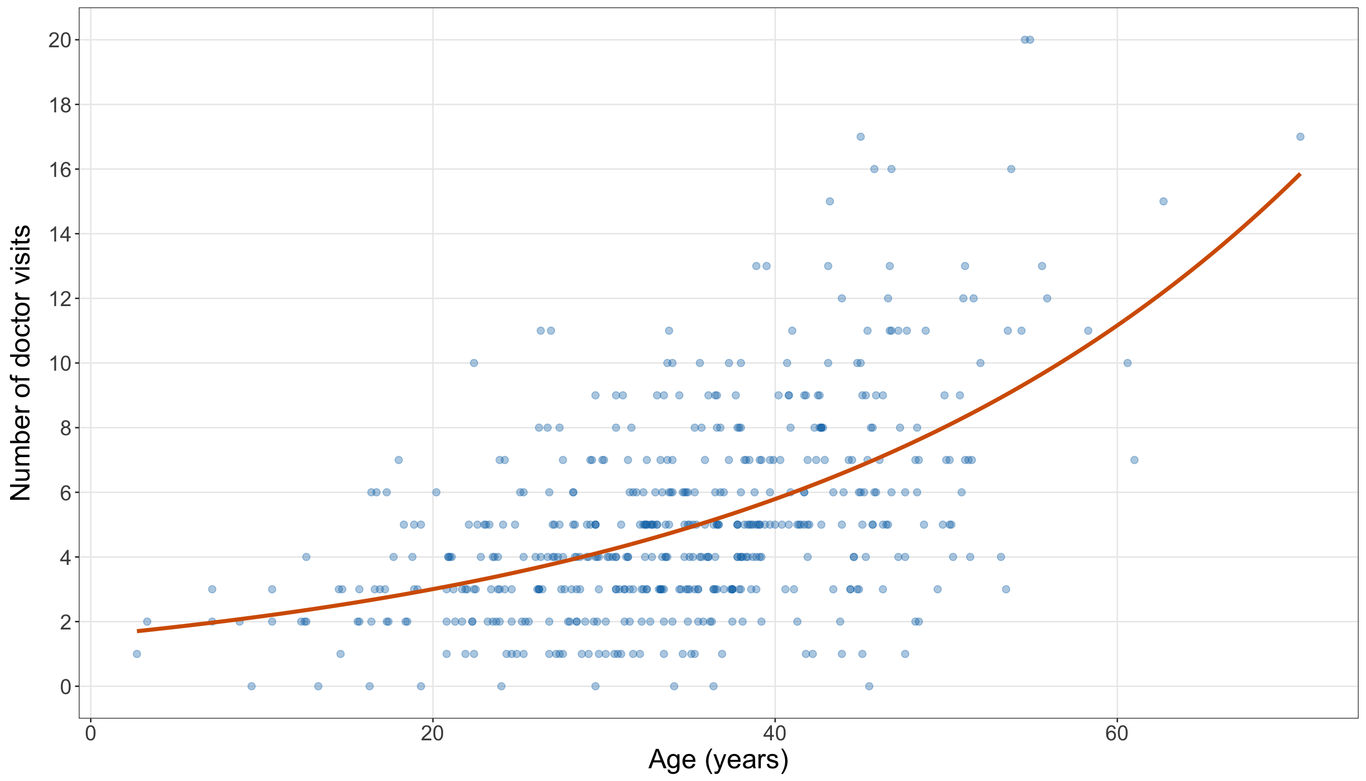
import matplotlib.pyplot as plt

# Creating the diagnostic quantities
doctor_simple_poisson_gof_data = (
    doctor_training_data.copy()
)

doctor_simple_poisson_gof_data[
    "fitted_expected_count"
] = doctor_simple_poisson_model.fittedvalues

doctor_simple_poisson_gof_data[
    "pearson_residual"
] = (
    doctor_simple_poisson_gof_data["doctor_visits"]
    - doctor_simple_poisson_gof_data[
        "fitted_expected_count"
    ]
) / np.sqrt(
    doctor_simple_poisson_gof_data[
        "fitted_expected_count"
    ]
)

doctor_simple_poisson_gof_data[
    "fitted_zero_probability"
] = np.exp(
    -doctor_simple_poisson_gof_data[
        "fitted_expected_count"
    ]
)

# Creating a smooth age grid for the fitted mean curve
doctor_simple_age_grid = pd.DataFrame(
    {
        "age": np.linspace(
            doctor_training_data["age"].min(),
            doctor_training_data["age"].max(),
            300,
        )
    }
)

doctor_simple_age_grid[
    "fitted_expected_count"
] = doctor_simple_poisson_model.predict(
    doctor_simple_age_grid
)

# Plotting observations and the fitted expected-count curve
(
    doctor_simple_age_curve_figure,
    doctor_simple_age_curve_axis,
) = plt.subplots(
    figsize=(14, 8)
)

_ = doctor_simple_age_curve_axis.scatter(
    doctor_training_data["age"],
    doctor_training_data["doctor_visits"],
    alpha=0.35,
    s=32,
    color="#0072B2",
)

_ = doctor_simple_age_curve_axis.plot(
    doctor_simple_age_grid["age"],
    doctor_simple_age_grid[
        "fitted_expected_count"
    ],
    linewidth=2.2,
    color="#D55E00",
)

_ = doctor_simple_age_curve_axis.set_xlabel(
    "Age (years)",
    fontsize=20,
)

_ = doctor_simple_age_curve_axis.set_ylabel(
    "Number of doctor visits",
    fontsize=20,
    labelpad=12,
)

_ = doctor_simple_age_curve_axis.set_yticks(
    range(
        0,
        int(doctor_training_data["doctor_visits"].max()) + 1,
        2,
    )
)

doctor_simple_age_curve_axis.tick_params(
    axis="both",
    labelsize=15.5,
)

doctor_simple_age_curve_axis.grid(
    True,
    which="major",
    axis="both",
    alpha=0.3,
)

doctor_simple_age_curve_axis.grid(
    False,
    which="minor",
)

doctor_simple_age_curve_figure.tight_layout()
plt.show()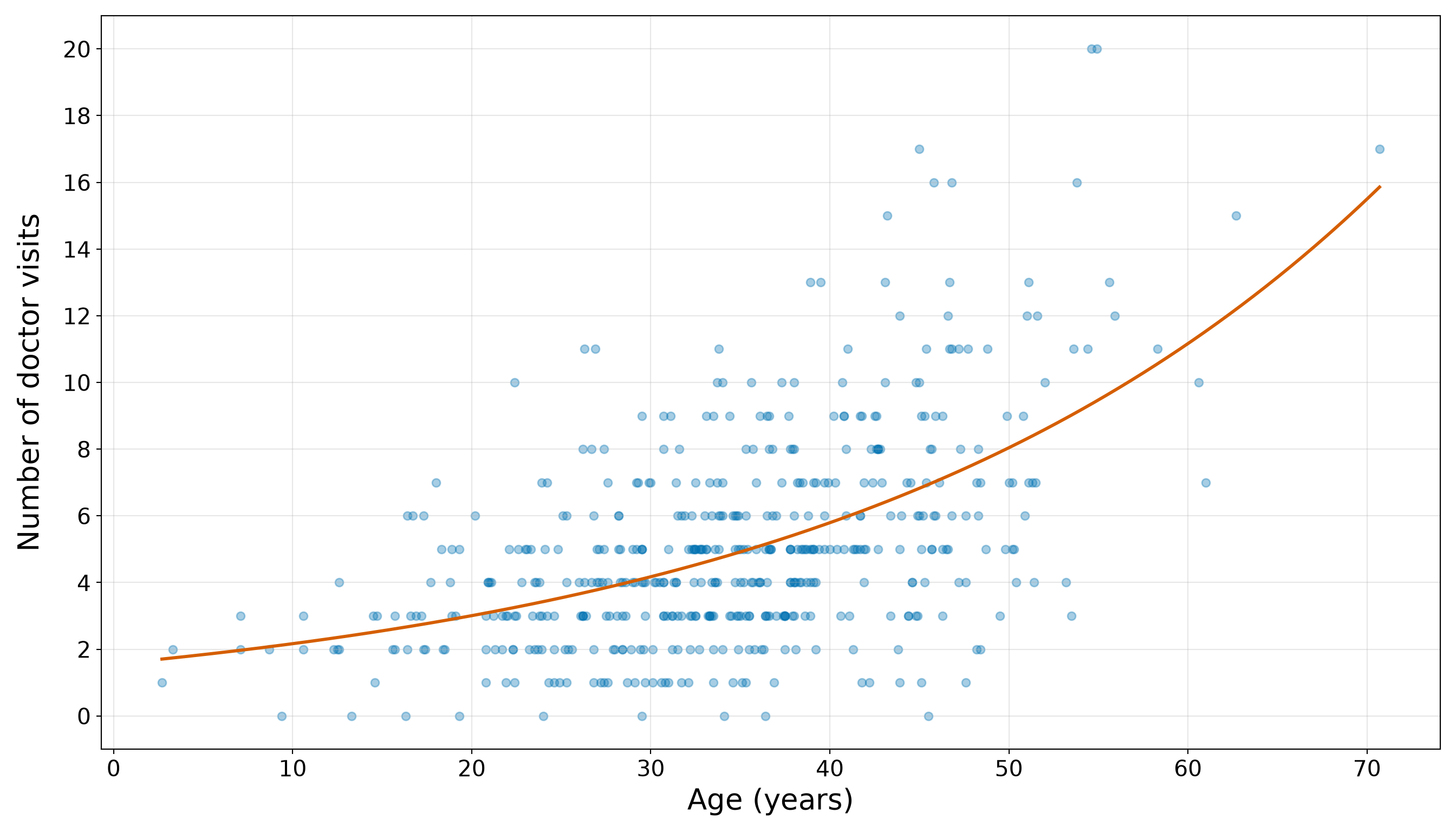
Figure 10.26 (or Figure 10.27) show a steadily increasing fitted expected count as age increases. This agrees with the EDA and the positive fitted age coefficient. However, the observed counts remain widely dispersed around the curve. At similar ages, some individuals report relatively few visits while others report substantially more. Therefore, the fitted mean trend can be useful even when the simple model does not reproduce the full conditional distribution.
Next, we group observations by their fitted expected counts. Since the age coefficient is positive, the first fitted-count quartile contains the smallest fitted expected counts and generally younger individuals, while the fourth contains the largest fitted expected counts and generally older individuals. This grouped comparison is a descriptive calibration check on the training data, not a held-out prediction assessment.
# Summarizing observations across fitted-count quartiles
doctor_simple_calibration <-
  doctor_simple_poisson_gof_data |>
  mutate(
    fitted_count_quartile = ntile(
      fitted_expected_count,
      4
    ),
    fitted_count_quartile = factor(
      fitted_count_quartile,
      levels = 1:4,
      labels = c(
        "Q1: smallest fitted counts",
        "Q2",
        "Q3",
        "Q4: largest fitted counts"
      )
    )
  ) |>
  group_by(fitted_count_quartile) |>
  summarize(
    number_of_individuals = n(),
    mean_age = mean(age),
    mean_observed_count = mean(doctor_visits),
    mean_fitted_count = mean(fitted_expected_count),
    observed_minus_fitted =
      mean_observed_count - mean_fitted_count,
    observed_zero_proportion = mean(
      doctor_visits == 0
    ),
    mean_fitted_zero_probability = mean(
      fitted_zero_probability
    ),
    .groups = "drop"
  )

# Formatting only for display
doctor_simple_calibration_display <-
  doctor_simple_calibration |>
  mutate(
    across(
      c(
        mean_age,
        mean_observed_count,
        mean_fitted_count,
        observed_minus_fitted,
        observed_zero_proportion,
        mean_fitted_zero_probability
      ),
      ~ formatC(
        .x,
        format = "f",
        digits = 3
      )
    )
  )

doctor_simple_calibration_display |>
  rename(
    `Fitted-count quartile` = fitted_count_quartile,
    `Number of individuals` = number_of_individuals,
    `Mean age` = mean_age,
    `Mean observed count` = mean_observed_count,
    `Mean fitted count` = mean_fitted_count,
    `Observed minus fitted` = observed_minus_fitted,
    `Observed zero proportion` = observed_zero_proportion,
    `Mean fitted zero probability` = mean_fitted_zero_probability
  ) |>
  kable(
    align = rep(
      "c",
      ncol(doctor_simple_calibration_display)
    )
)| Fitted-count quartile | Number of individuals | Mean age | Mean observed count | Mean fitted count | Observed minus fitted | Observed zero proportion | Mean fitted zero probability |
|---|---|---|---|---|---|---|---|
| Q1: smallest fitted counts | 125 | 21.326 | 3.400 | 3.187 | 0.213 | 0.040 | 0.048 |
| Q2 | 125 | 31.454 | 4.320 | 4.385 | -0.065 | 0.016 | 0.013 |
| Q3 | 125 | 37.485 | 5.160 | 5.343 | -0.183 | 0.008 | 0.005 |
| Q4: largest fitted counts | 125 | 47.031 | 7.432 | 7.398 | 0.034 | 0.008 | 0.001 |
# Reproducing dplyr::ntile() for four equal-sized groups
doctor_fitted_rank = doctor_simple_poisson_gof_data[
    "fitted_expected_count"
].rank(method="first")

doctor_simple_poisson_gof_data[
    "fitted_count_quartile_number"
] = np.ceil(
    4 * doctor_fitted_rank
    / len(doctor_simple_poisson_gof_data)
).astype(int)

doctor_fitted_quartile_labels = {
    1: "Q1: smallest fitted counts",
    2: "Q2",
    3: "Q3",
    4: "Q4: largest fitted counts",
}

doctor_simple_poisson_gof_data[
    "fitted_count_quartile"
] = doctor_simple_poisson_gof_data[
    "fitted_count_quartile_number"
].map(doctor_fitted_quartile_labels)

# Summarizing observations across fitted-count quartiles
doctor_simple_calibration = (
    doctor_simple_poisson_gof_data
    .groupby(
        "fitted_count_quartile_number",
        sort=True,
    )
    .agg(
        number_of_individuals=(
            "doctor_visits",
            "size",
        ),
        mean_age=(
            "age",
            "mean",
        ),
        mean_observed_count=(
            "doctor_visits",
            "mean",
        ),
        mean_fitted_count=(
            "fitted_expected_count",
            "mean",
        ),
        observed_zero_proportion=(
            "doctor_visits",
            lambda values: (values == 0).mean(),
        ),
        mean_fitted_zero_probability=(
            "fitted_zero_probability",
            "mean",
        ),
    )
    .reset_index()
)

doctor_simple_calibration[
    "observed_minus_fitted"
] = (
    doctor_simple_calibration[
        "mean_observed_count"
    ]
    - doctor_simple_calibration[
        "mean_fitted_count"
    ]
)

doctor_simple_calibration[
    "Fitted-count quartile"
] = doctor_simple_calibration[
    "fitted_count_quartile_number"
].map(doctor_fitted_quartile_labels)

# Formatting only for display
doctor_simple_calibration_display = (
    doctor_simple_calibration[
        [
            "Fitted-count quartile",
            "number_of_individuals",
            "mean_age",
            "mean_observed_count",
            "mean_fitted_count",
            "observed_minus_fitted",
            "observed_zero_proportion",
            "mean_fitted_zero_probability",
        ]
    ]
    .rename(
        columns={
            "number_of_individuals": "Number of individuals",
            "mean_age": "Mean age",
            "mean_observed_count": "Mean observed count",
            "mean_fitted_count": "Mean fitted count",
            "observed_minus_fitted": "Observed minus fitted",
            "observed_zero_proportion": "Observed zero proportion",
            "mean_fitted_zero_probability": (
                "Mean fitted zero probability"
            ),
        }
    )
    .copy()
)

for column in [
    "Mean age",
    "Mean observed count",
    "Mean fitted count",
    "Observed minus fitted",
    "Observed zero proportion",
    "Mean fitted zero probability",
]:
    doctor_simple_calibration_display[column] = (
        doctor_simple_calibration_display[column]
        .map(lambda value: f"{value:.3f}")
    )

doctor_simple_calibration_html = (
    doctor_simple_calibration_display.to_html(
        index=False,
        border=0,
    )
)| Fitted-count quartile | Number of individuals | Mean age | Mean observed count | Mean fitted count | Observed minus fitted | Observed zero proportion | Mean fitted zero probability |
|---|---|---|---|---|---|---|---|
| Q1: smallest fitted counts | 125 | 21.326 | 3.400 | 3.187 | 0.213 | 0.040 | 0.048 |
| Q2 | 125 | 31.454 | 4.320 | 4.385 | -0.065 | 0.016 | 0.013 |
| Q3 | 125 | 37.485 | 5.160 | 5.343 | -0.183 | 0.008 | 0.005 |
| Q4: largest fitted counts | 125 | 47.031 | 7.432 | 7.398 | 0.034 | 0.008 | 0.001 |
In Table 10.99, the grouped means show that the simple model captures the broad ordering associated with age. In the first fitted-count quartile, the mean observed count is 3.400, compared with a mean fitted count of 3.187. In the fourth quartile, the corresponding values are 7.432 and 7.398. Thus, the fitted mean rises in the same direction as the grouped observed mean.
Nevertheless, closeness of grouped means is not enough to establish model adequacy. Individuals within the same fitted-count range can still show much more variability than the Classical Poisson distribution permits. The zero-proportion columns also provide a preliminary comparison between observed and fitted zero behaviour, which will be assessed more directly in Question 10.38.
The following observed-versus-fitted plot makes the individual-level discrepancies visible. The dashed line marks the location where an observed count would equal its fitted expected count.
# Common axis limit for the observed-versus-fitted comparison
doctor_simple_observed_fitted_limit <- max(
  doctor_simple_poisson_gof_data$doctor_visits,
  doctor_simple_poisson_gof_data$fitted_expected_count
)

# Plotting observed counts against fitted expected counts
doctor_simple_observed_fitted_plot <- ggplot(
  doctor_simple_poisson_gof_data,
  aes(
    x = fitted_expected_count,
    y = doctor_visits
  )
) +
  geom_abline(
    intercept = 0,
    slope = 1,
    linetype = "dashed",
    linewidth = 1,
    colour = "#D55E00"
  ) +
  geom_point(
    alpha = 0.45,
    size = 2.3,
    colour = "#0072B2"
  ) +
  coord_equal(
    xlim = c(0, doctor_simple_observed_fitted_limit),
    ylim = c(0, doctor_simple_observed_fitted_limit)
  ) +
  theme_bw() +
  theme(
    axis.text = element_text(size = 15.5),
    axis.title.x = element_text(size = 20),
    axis.title.y = element_text(
      size = 20,
      vjust = 0.5,
      margin = margin(r = 12)
    ),
    panel.grid.minor = element_blank()
  ) +
  labs(
    x = "Fitted expected count",
    y = "Observed doctor visits"
  )

doctor_simple_observed_fitted_plot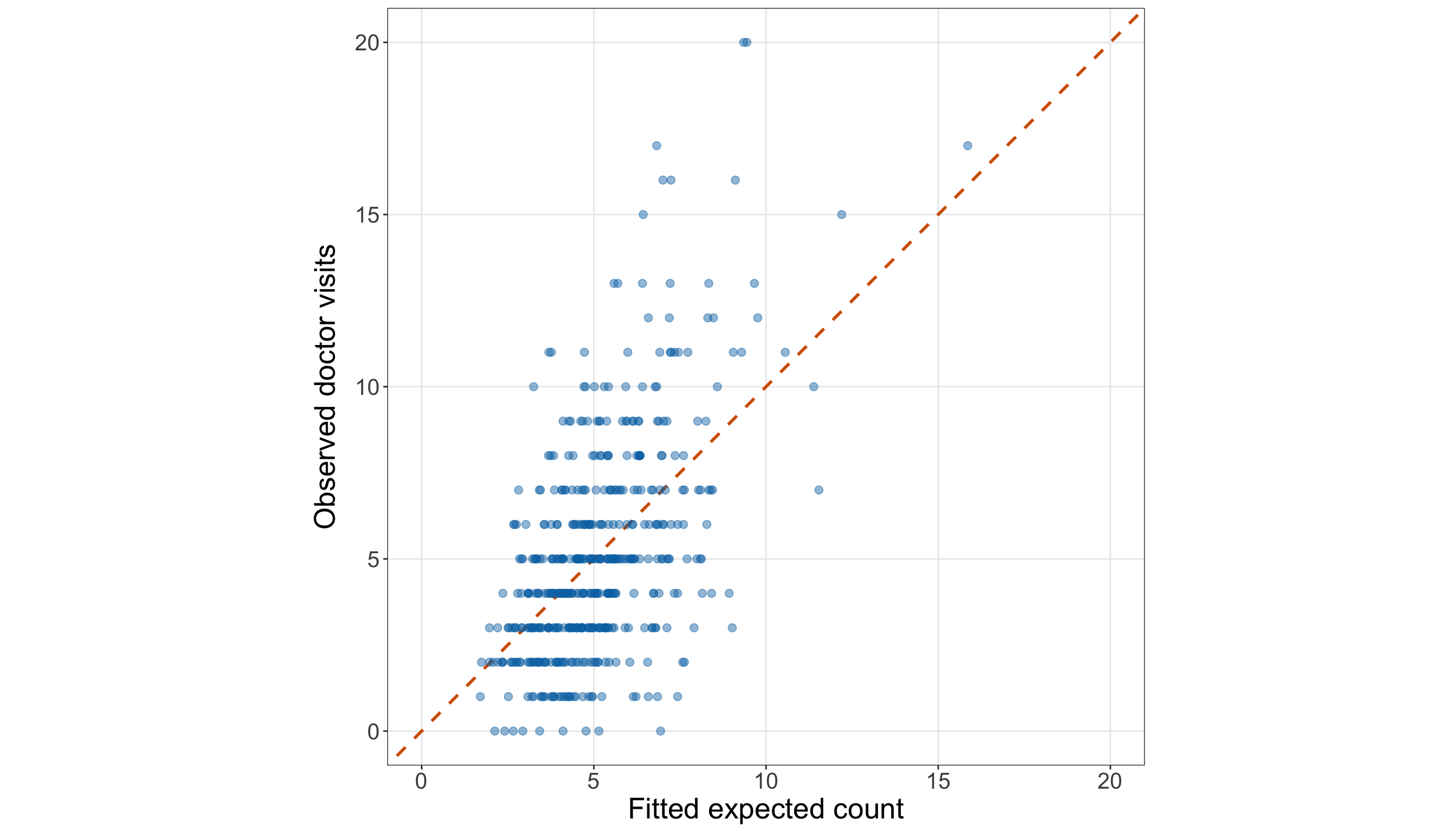
# Common axis limit for the observed-versus-fitted comparison
doctor_simple_observed_fitted_limit = max(
    doctor_simple_poisson_gof_data[
        "doctor_visits"
    ].max(),
    doctor_simple_poisson_gof_data[
        "fitted_expected_count"
    ].max(),
)

# Plotting observed counts against fitted expected counts
(
    doctor_simple_observed_fitted_figure,
    doctor_simple_observed_fitted_axis,
) = plt.subplots(
    figsize=(14, 8)
)

_ = doctor_simple_observed_fitted_axis.plot(
    [0, doctor_simple_observed_fitted_limit],
    [0, doctor_simple_observed_fitted_limit],
    linestyle="--",
    linewidth=1.5,
    color="#D55E00",
)

_ = doctor_simple_observed_fitted_axis.scatter(
    doctor_simple_poisson_gof_data[
        "fitted_expected_count"
    ],
    doctor_simple_poisson_gof_data[
        "doctor_visits"
    ],
    alpha=0.45,
    s=35,
    color="#0072B2",
)

_ = doctor_simple_observed_fitted_axis.set_xlim(
    0,
    doctor_simple_observed_fitted_limit,
)

_ = doctor_simple_observed_fitted_axis.set_ylim(
    0,
    doctor_simple_observed_fitted_limit,
)

_ = doctor_simple_observed_fitted_axis.set_aspect(
    "equal",
    adjustable="box",
)

_ = doctor_simple_observed_fitted_axis.set_xlabel(
    "Fitted expected count",
    fontsize=20,
)

_ = doctor_simple_observed_fitted_axis.set_ylabel(
    "Observed doctor visits",
    fontsize=20,
    labelpad=12,
)

doctor_simple_observed_fitted_axis.tick_params(
    axis="both",
    labelsize=15.5,
)

doctor_simple_observed_fitted_axis.grid(
    True,
    which="major",
    axis="both",
    alpha=0.3,
)

doctor_simple_observed_fitted_axis.grid(
    False,
    which="minor",
)

doctor_simple_observed_fitted_figure.tight_layout()
plt.show()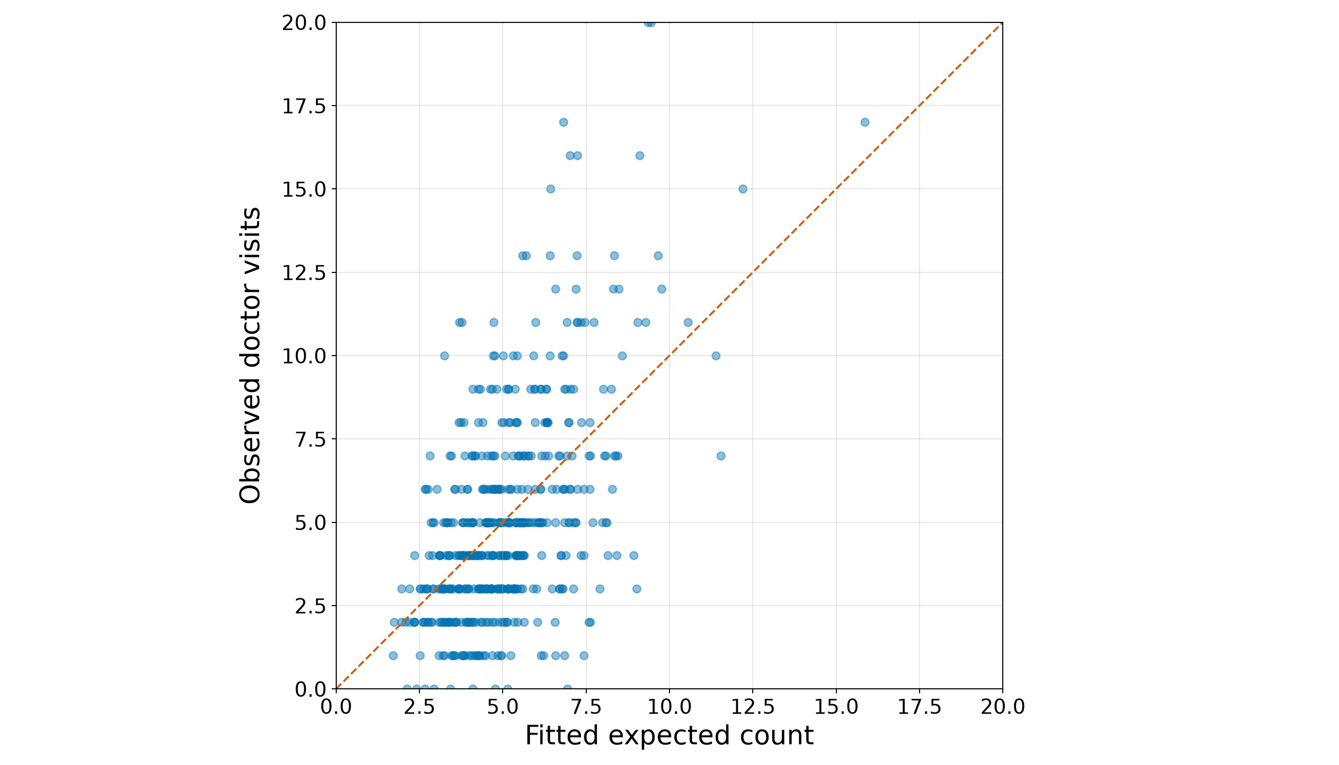
The fitted expected counts range from 1.704 to 15.858, while the observed counts range from 0 to 20. Hence, the model produces a comparatively narrow band of fitted means, but individuals with similar fitted means exhibit a much broader range of observed counts. Figure 10.28 (or Figure 10.29) therefore suggests that age captures an important mean trend without fully accounting for the training-set variability.
Question 10.38 — Checking the Simple Model’s Distributional Fit
For the simple age-only Classical Poisson regression:
- Compute the Pearson Chi-squared statistic, residual degrees of freedom, Pearson dispersion estimate, and one-sided overdispersion \(p\)-value.
- Compare the observed number of zero visits with the fitted expected number of zeros. Then, compute the approximate zero-count \(z\)-statistic and its one-sided \(p\)-value.
- Compute the residual deviance, residual degrees of freedom, residual-deviance ratio, and goodness-of-fit \(p\)-value.
- Construct a Pearson-residual-versus-fitted plot with horizontal reference lines at \(0\), \(-2\), and \(2\).
- Interpret the checks jointly. Distinguish evidence of general lack of fit or overdispersion from evidence specifically concerning excess zeros.
Answer 10.38
Click here to reveal the answer!
We begin with the Pearson dispersion check developed in Section 10.8.2. The Pearson Chi-squared statistic is defined in Equation 10.14, and the dispersion estimate is defined in Equation 10.15. For the one-sided overdispersion check, the working hypotheses are
\[ H_0: \phi = 1 \qquad \text{versus} \qquad H_A: \phi > 1. \]
A dispersion estimate appreciably above \(1\), together with a small upper-tail \(p\)-value, indicates that the counts vary more around the fitted mean than the Classical Poisson model permits.
# Pearson Chi-squared statistic
doctor_simple_pearson_chi_squared <- sum(
  residuals(
    doctor_simple_poisson_model,
    type = "pearson"
  )^2
)

# Residual degrees of freedom
doctor_simple_pearson_df <- df.residual(
  doctor_simple_poisson_model
)

# Pearson dispersion estimate
doctor_simple_pearson_dispersion <-
  doctor_simple_pearson_chi_squared /
  doctor_simple_pearson_df

# One-sided upper-tail p-value
doctor_simple_pearson_p_value <- pchisq(
  doctor_simple_pearson_chi_squared,
  df = doctor_simple_pearson_df,
  lower.tail = FALSE
)

# Summary table
doctor_simple_pearson_summary <- tibble(
  quantity = c(
    "Pearson Chi-squared statistic",
    "Residual degrees of freedom",
    "Pearson dispersion estimate",
    "One-sided overdispersion p-value"
  ),
  value = c(
    formatC(
      doctor_simple_pearson_chi_squared,
      format = "f",
      digits = 3
    ),
    formatC(
      doctor_simple_pearson_df,
      format = "f",
      digits = 0
    ),
    formatC(
      doctor_simple_pearson_dispersion,
      format = "f",
      digits = 3
    ),
    formatC(
      doctor_simple_pearson_p_value,
      format = "e",
      digits = 2
    )
  )
)

doctor_simple_pearson_summary |>
  rename(
    `Quantity` = quantity,
    `Value` = value
  ) |>
  kable(
    align = c("c", "c")
)| Quantity | Value |
|---|---|
| Pearson Chi-squared statistic | 656.139 |
| Residual degrees of freedom | 498 |
| Pearson dispersion estimate | 1.318 |
| One-sided overdispersion p-value | 2.31e-06 |
from scipy import stats

# Pearson Chi-squared statistic
doctor_simple_pearson_chi_squared = np.sum(
    doctor_simple_poisson_model.resid_pearson ** 2
)

# Residual degrees of freedom
doctor_simple_pearson_df = (
    doctor_simple_poisson_model.df_resid
)

# Pearson dispersion estimate
doctor_simple_pearson_dispersion = (
    doctor_simple_pearson_chi_squared
    / doctor_simple_pearson_df
)

# One-sided upper-tail p-value
doctor_simple_pearson_p_value = stats.chi2.sf(
    doctor_simple_pearson_chi_squared,
    doctor_simple_pearson_df,
)

# Summary table
doctor_simple_pearson_summary = pd.DataFrame(
    {
        "Quantity": [
            "Pearson Chi-squared statistic",
            "Residual degrees of freedom",
            "Pearson dispersion estimate",
            "One-sided overdispersion p-value",
        ],
        "Value": [
            f"{doctor_simple_pearson_chi_squared:.3f}",
            f"{doctor_simple_pearson_df:.0f}",
            f"{doctor_simple_pearson_dispersion:.3f}",
            f"{doctor_simple_pearson_p_value:.2e}",
        ],
    }
)

doctor_simple_pearson_summary_html = (
    doctor_simple_pearson_summary.to_html(
        index=False,
        border=0,
    )
)| Quantity | Value |
|---|---|
| Pearson Chi-squared statistic | 656.139 |
| Residual degrees of freedom | 498 |
| Pearson dispersion estimate | 1.318 |
| One-sided overdispersion p-value | 2.31e-06 |
The Pearson dispersion estimate is 1.318, and the one-sided overdispersion \(p\)-value is 2.31e-06. At the 5% significance level, this provides evidence that the conditional variability remaining around the age-only fitted mean is larger than the Classical Poisson model allows.
This diagnostic is critical for more than model fit. Under overdispersion, the Classical Poisson model-based standard errors can be too small because they are calculated under the restrictive conditional variance assumption
\[\operatorname{Var}(Y_i \mid x_{i,1}) = \mu_i.\]
Next, we isolate the zero-count component. For each observation, the fitted probability of zero visits is \(\exp(-\hat\mu_i)\). Adding these probabilities gives the fitted expected number of zeros. The approximate \(z\)-statistic follows Equation 10.16. The hypotheses are the following:
\[ \begin{gather} H_0\text{: } \text{the fitted Classical Poisson model adequately describes} \\ \text{the frequency of zero counts}, \\ \text{versus} \\ H_1\text{: } \text{there are more zero counts than the} \\ \text{fitted Classical Poisson model expects}. \end{gather} \]
# Observed and fitted expected numbers of zeros
doctor_simple_observed_zero_count <- sum(
  doctor_simple_poisson_gof_data$doctor_visits == 0
)

doctor_simple_expected_zero_count <- sum(
  doctor_simple_poisson_gof_data$fitted_zero_probability
)

# Variance of the fitted sum of unequal-probability Bernoulli indicators
doctor_simple_zero_count_variance <- sum(
  doctor_simple_poisson_gof_data$fitted_zero_probability *
    (
      1 -
      doctor_simple_poisson_gof_data$fitted_zero_probability
    )
)

# Approximate one-sided z-test
doctor_simple_zero_count_z <- (
  doctor_simple_observed_zero_count -
    doctor_simple_expected_zero_count
) / sqrt(doctor_simple_zero_count_variance)

doctor_simple_zero_count_p_value <- pnorm(
  doctor_simple_zero_count_z,
  lower.tail = FALSE
)

# Summary table
doctor_simple_zero_count_summary <- tibble(
  quantity = c(
    "Observed zero count",
    "Fitted expected zero count",
    "Observed minus fitted zeros",
    "Approximate z-statistic",
    "One-sided p-value"
  ),
  value = c(
    formatC(
      doctor_simple_observed_zero_count,
      format = "f",
      digits = 0
    ),
    formatC(
      doctor_simple_expected_zero_count,
      format = "f",
      digits = 2
    ),
    formatC(
      doctor_simple_observed_zero_count -
        doctor_simple_expected_zero_count,
      format = "f",
      digits = 2
    ),
    formatC(
      doctor_simple_zero_count_z,
      format = "f",
      digits = 2
    ),
    formatC(
      doctor_simple_zero_count_p_value,
      format = "e",
      digits = 2
    )
  )
)

doctor_simple_zero_count_summary |>
  rename(
    `Quantity` = quantity,
    `Value` = value
  ) |>
  kable(
    align = c("c", "c")
)| Quantity | Value |
|---|---|
| Observed zero count | 9 |
| Fitted expected zero count | 8.37 |
| Observed minus fitted zeros | 0.63 |
| Approximate z-statistic | 0.22 |
| One-sided p-value | 4.12e-01 |
# Observed and fitted expected numbers of zeros
doctor_simple_observed_zero_count = (
    doctor_simple_poisson_gof_data[
        "doctor_visits"
    ]
    == 0
).sum()

doctor_simple_expected_zero_count = (
    doctor_simple_poisson_gof_data[
        "fitted_zero_probability"
    ].sum()
)

# Variance of the fitted sum of unequal-probability Bernoulli indicators
doctor_simple_zero_count_variance = (
    doctor_simple_poisson_gof_data[
        "fitted_zero_probability"
    ]
    * (
        1
        - doctor_simple_poisson_gof_data[
            "fitted_zero_probability"
        ]
    )
).sum()

# Approximate one-sided z-test
doctor_simple_zero_count_z = (
    doctor_simple_observed_zero_count
    - doctor_simple_expected_zero_count
) / np.sqrt(doctor_simple_zero_count_variance)

doctor_simple_zero_count_p_value = stats.norm.sf(
    doctor_simple_zero_count_z
)

# Summary table
doctor_simple_zero_count_summary = pd.DataFrame(
    {
        "Quantity": [
            "Observed zero count",
            "Fitted expected zero count",
            "Observed minus fitted zeros",
            "Approximate z-statistic",
            "One-sided p-value",
        ],
        "Value": [
            f"{doctor_simple_observed_zero_count:.0f}",
            f"{doctor_simple_expected_zero_count:.2f}",
            f"{doctor_simple_observed_zero_count - doctor_simple_expected_zero_count:.2f}",
            f"{doctor_simple_zero_count_z:.2f}",
            f"{doctor_simple_zero_count_p_value:.2e}",
        ],
    }
)

doctor_simple_zero_count_summary_html = (
    doctor_simple_zero_count_summary.to_html(
        index=False,
        border=0,
    )
)| Quantity | Value |
|---|---|
| Observed zero count | 9 |
| Fitted expected zero count | 8.37 |
| Observed minus fitted zeros | 0.63 |
| Approximate z-statistic | 0.22 |
| One-sided p-value | 4.12e-01 |
The training data contain 9 observed zero counts, while the simple fitted model expects 8.37 zeros. The difference is 0.63, and the one-sided \(p\)-value is 4.12e-01. This does not provide strong evidence that excess zeros are a primary source of the age-only model’s lack of fit (i.e., we fail to reject the null hypothesis). Note that this distinction is important. A model can show overdispersion or global lack of fit even when its zero-count frequency is not unusually poor. Therefore, we should avoid treating every inadequate Poisson model as automatically requiring a zero-inflated alternative.
Finally, we calculate the residual deviance from Equation 10.18. Under an adequate fitted model, the residual deviance is commonly compared with a Chi-squared reference distribution using the residual degrees of freedom. Recall that the hypotheses are the following:
\[ \begin{gather} H_0\text{: } \text{the fitted Classical Poisson model is adequate}, \\ \text{versus} \\ H_1\text{: } \text{the fitted Classical Poisson model is not adequate}. \end{gather} \]
A large residual-deviance ratio and a small upper-tail \(p\)-value indicate global lack of fit relative to the saturated benchmark.
# Residual deviance and degrees of freedom
doctor_simple_residual_deviance <- deviance(
  doctor_simple_poisson_model
)

doctor_simple_residual_deviance_df <- df.residual(
  doctor_simple_poisson_model
)

# Residual-deviance ratio
doctor_simple_residual_deviance_ratio <-
  doctor_simple_residual_deviance /
  doctor_simple_residual_deviance_df

# Upper-tail goodness-of-fit p-value
doctor_simple_residual_deviance_p_value <- pchisq(
  doctor_simple_residual_deviance,
  df = doctor_simple_residual_deviance_df,
  lower.tail = FALSE
)

# Summary table
doctor_simple_residual_deviance_summary <- tibble(
  quantity = c(
    "Residual deviance",
    "Residual degrees of freedom",
    "Residual deviance / df",
    "Goodness-of-fit p-value"
  ),
  value = c(
    formatC(
      doctor_simple_residual_deviance,
      format = "f",
      digits = 3
    ),
    formatC(
      doctor_simple_residual_deviance_df,
      format = "f",
      digits = 0
    ),
    formatC(
      doctor_simple_residual_deviance_ratio,
      format = "f",
      digits = 3
    ),
    formatC(
      doctor_simple_residual_deviance_p_value,
      format = "e",
      digits = 2
    )
  )
)

doctor_simple_residual_deviance_summary |>
  rename(
    `Quantity` = quantity,
    `Value` = value
  ) |>
  kable(
    align = c("c", "c")
)| Quantity | Value |
|---|---|
| Residual deviance | 675.525 |
| Residual degrees of freedom | 498 |
| Residual deviance / df | 1.356 |
| Goodness-of-fit p-value | 1.80e-07 |
# Residual deviance and degrees of freedom
doctor_simple_residual_deviance = (
    doctor_simple_poisson_model.deviance
)

doctor_simple_residual_deviance_df = (
    doctor_simple_poisson_model.df_resid
)

# Residual-deviance ratio
doctor_simple_residual_deviance_ratio = (
    doctor_simple_residual_deviance
    / doctor_simple_residual_deviance_df
)

# Upper-tail goodness-of-fit p-value
doctor_simple_residual_deviance_p_value = stats.chi2.sf(
    doctor_simple_residual_deviance,
    doctor_simple_residual_deviance_df,
)

# Summary table
doctor_simple_residual_deviance_summary = pd.DataFrame(
    {
        "Quantity": [
            "Residual deviance",
            "Residual degrees of freedom",
            "Residual deviance / df",
            "Goodness-of-fit p-value",
        ],
        "Value": [
            f"{doctor_simple_residual_deviance:.3f}",
            f"{doctor_simple_residual_deviance_df:.0f}",
            f"{doctor_simple_residual_deviance_ratio:.3f}",
            f"{doctor_simple_residual_deviance_p_value:.2e}",
        ],
    }
)

doctor_simple_residual_deviance_summary_html = (
    doctor_simple_residual_deviance_summary.to_html(
        index=False,
        border=0,
    )
)| Quantity | Value |
|---|---|
| Residual deviance | 675.525 |
| Residual degrees of freedom | 498 |
| Residual deviance / df | 1.356 |
| Goodness-of-fit p-value | 1.80e-07 |
The residual deviance is 675.525 on 498 residual degrees of freedom, giving a residual-deviance ratio of 1.356. The corresponding goodness-of-fit \(p\)-value is 1.80e-07. This provides global evidence that the simple age-only Classical Poisson model does not reproduce the training counts adequately.
A residual plot helps show how the discrepancies are distributed. The dashed lines at \(-2\) and \(2\) are informal reference bands rather than formal decision thresholds. We also count the observations outside these bands so that the interpretation is tied to the rendered output.
# Residual counts used in the interpretation
doctor_simple_large_positive_residuals <- sum(
  doctor_simple_poisson_gof_data$pearson_residual > 2
)

doctor_simple_large_negative_residuals <- sum(
  doctor_simple_poisson_gof_data$pearson_residual < -2
)

doctor_simple_maximum_absolute_residual <- max(
  abs(doctor_simple_poisson_gof_data$pearson_residual)
)

# Plotting Pearson residuals against fitted expected counts
doctor_simple_pearson_residual_plot <- ggplot(
  doctor_simple_poisson_gof_data,
  aes(
    x = fitted_expected_count,
    y = pearson_residual
  )
) +
  geom_hline(
    yintercept = 0,
    linewidth = 0.8,
    colour = "grey40"
  ) +
  geom_hline(
    yintercept = c(-2, 2),
    linetype = "dashed",
    linewidth = 0.8,
    colour = "#D55E00"
  ) +
  geom_point(
    alpha = 0.60,
    size = 2.3,
    colour = "#0072B2"
  ) +
  theme_bw() +
  theme(
    axis.text = element_text(size = 15.5),
    axis.title.x = element_text(size = 20),
    axis.title.y = element_text(
      size = 20,
      vjust = 0.5,
      margin = margin(r = 12)
    ),
    panel.grid.minor = element_blank()
  ) +
  labs(
    x = "Fitted expected count",
    y = "Pearson residual"
  )

doctor_simple_pearson_residual_plot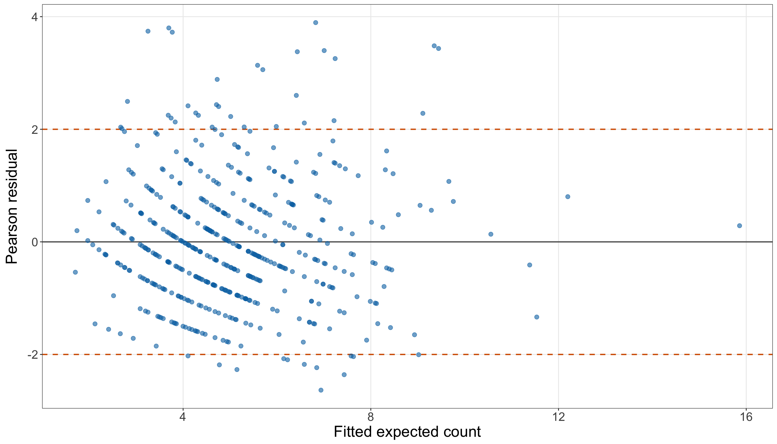
# Residual counts used in the interpretation
doctor_simple_large_positive_residuals = (
    doctor_simple_poisson_gof_data[
        "pearson_residual"
    ]
    > 2
).sum()

doctor_simple_large_negative_residuals = (
    doctor_simple_poisson_gof_data[
        "pearson_residual"
    ]
    < -2
).sum()

doctor_simple_maximum_absolute_residual = np.abs(
    doctor_simple_poisson_gof_data[
        "pearson_residual"
    ]
).max()

# Plotting Pearson residuals against fitted expected counts
(
    doctor_simple_pearson_residual_figure,
    doctor_simple_pearson_residual_axis,
) = plt.subplots(
    figsize=(14, 8)
)

_ = doctor_simple_pearson_residual_axis.axhline(
    0,
    linewidth=0.8,
    color="grey",
)

_ = doctor_simple_pearson_residual_axis.axhline(
    2,
    linestyle="--",
    linewidth=0.8,
    color="#D55E00",
)

_ = doctor_simple_pearson_residual_axis.axhline(
    -2,
    linestyle="--",
    linewidth=0.8,
    color="#D55E00",
)

_ = doctor_simple_pearson_residual_axis.scatter(
    doctor_simple_poisson_gof_data[
        "fitted_expected_count"
    ],
    doctor_simple_poisson_gof_data[
        "pearson_residual"
    ],
    alpha=0.60,
    s=35,
    color="#0072B2",
)

_ = doctor_simple_pearson_residual_axis.set_xlabel(
    "Fitted expected count",
    fontsize=20,
)

_ = doctor_simple_pearson_residual_axis.set_ylabel(
    "Pearson residual",
    fontsize=20,
    labelpad=12,
)

doctor_simple_pearson_residual_axis.tick_params(
    axis="both",
    labelsize=15.5,
)

doctor_simple_pearson_residual_axis.grid(
    True,
    which="major",
    axis="both",
    alpha=0.3,
)

doctor_simple_pearson_residual_axis.grid(
    False,
    which="minor",
)

doctor_simple_pearson_residual_figure.tight_layout()
plt.show()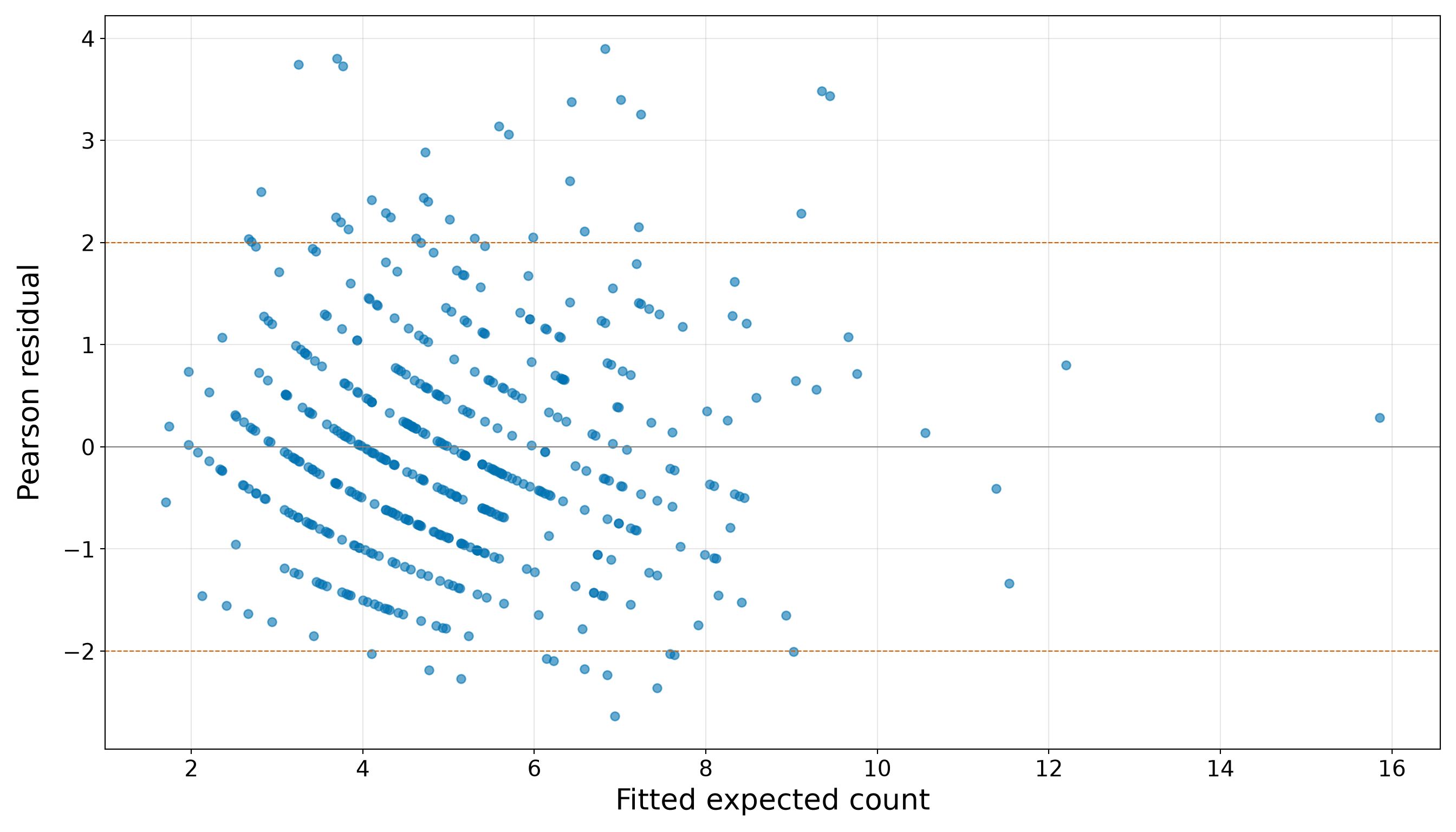
The residual plot in Figure 10.30 (or Figure 10.31) contains 31 Pearson residuals above \(2\) and 12 below \(-2\). The largest absolute Pearson residual is 3.895. These discrepancies reinforce the need to examine more than the fitted age trend alone. A model may track the average increase in counts with age while still understating how much individual counts vary around that trend.
Question 10.39 — Deciding Whether the Simple Model Is Adequate
Summarize the evidence from Questions 10.36 to 10.38:
- State what the age-only model captures successfully.
- State whether the Pearson dispersion and residual-deviance checks support the Classical Poisson distributional assumptions.
- State whether the zero-count check identifies excess zeros as a primary concern.
- Explain why the model should be extended before the case study proceeds to final inference and prediction.
- Identify the regressors that should be added in the extended model.
Answer 10.39
Click here to reveal the answer!
Table 10.107 brings together the simple-model evidence.
| Component | Training-set finding | Implication |
|---|---|---|
| Fitted age relationship | The fitted age multiplier is 1.0333 per year and 1.388 per ten years. The fitted expected count increases across the observed age range. | Age captures a clear and interpretable part of the conditional mean structure. |
| Grouped calibration | The first fitted-count quartile has mean observed and fitted counts of 3.400 and 3.187, while the fourth has 7.432 and 7.398. | The model captures the broad increase in average visits with age, but grouped means do not assess the full conditional variability. |
| Pearson dispersion | The dispersion estimate is 1.318, with one-sided \(p\)-value 2.31e-06. | The remaining variability exceeds what the Classical Poisson variance assumption allows. |
| Zero counts | The training data contain 9 observed zeros, while the model expects 8.37. The one-sided \(p\)-value is 4.12e-01. | The diagnostic does not identify excess zeros as the main problem. |
| Residual deviance | The residual-deviance ratio is 1.356, with goodness-of-fit \(p\)-value 1.80e-07. | The age-only model shows global lack of fit relative to the saturated benchmark. |
| Pearson residuals | There are 31 residuals above \(2\) and 12 below \(-2\); the largest absolute residual is 3.895. | The fitted age trend does not fully represent the individual-level spread of annual doctor visits. |
The age-only model is useful because it translates the strongest EDA pattern into a clear fitted mean relationship. However, model adequacy depends on more than whether one coefficient has the expected sign or whether grouped fitted means broadly track grouped observed means.
At the 5% significance level, both the Pearson dispersion and residual-deviance checks indicate that the simple Classical Poisson model is too restrictive for the training data. In contrast, the zero-count check does not provide strong evidence that excess zeros are the main source of the discrepancy.
The next modelling step is therefore to revisit the systematic component before abandoning Classical Poisson regression altogether. The EDA identified additional structure associated with:
-
income; -
education_years; -
married; -
urban; and -
insurance.
The extended model will retain age and add these five explanatory variables. This will test whether part of the apparent overdispersion and global lack of fit arises because the age-only mean structure omits relevant demographic and socioeconomic information. After fitting the extended model, we must repeat the goodness-of-fit checks rather than assuming that additional regressors automatically solve the distributional concerns.
The testing set remains untouched. It will be used only after the extended-model development and diagnostic stages have been completed.
Extended Classical Poisson Regression and Goodness of Fit
The simple age-only model identified a meaningful age pattern, but its goodness-of-fit checks showed that age alone did not provide an adequate conditional description of the training counts. We now extend the systematic component by adding the demographic and socioeconomic regressors identified during EDA. The random component remains Classical Poisson, so the extension must still pass the same distributional checks before the case study proceeds to the results stage.
The workflow in this subsection remains confined to doctor_training_data. We will:
- specify and fit the extended model;
- examine fitted counts and grouped calibration;
- repeat the Pearson-dispersion, zero-count, residual-deviance, and residual checks; and
- decide whether the selected extended model is sufficiently adequate to move forward.
The testing set remains untouched throughout this subsection.
Question 10.40 — Specifying and Fitting the Extended Classical Poisson Regression
Using only doctor_training_data:
Rescale annual income into thousands of dollars and call the resulting regressor
income_1000.-
Specify an extended Classical Poisson regression containing:
-
age; -
income_1000; -
education_years; -
married; -
urban; and -
insurance.
-
Write the random component, systematic component, and log link mathematically. Recall that you need to define the dummy variables and identify the baseline categories.
Fit the model in
RandPythonon the common training set.Report the coefficient estimates, model-based standard errors, exponentiated estimates, and fitted percent changes.
Explain why this training-set table supports model development but does not yet provide the case study’s final inferential conclusions.
Answer 10.40
Click here to reveal the answer!
We rescale income because a one-dollar comparison would produce a very small coefficient and an exponentiated estimate extremely close to \(1\). Define
\[ x_{i,2} = \frac{\text{annual income of individual }i}{1{,}000}. \]
A one-unit increase in \(x_{i,2}\) therefore represents a \(\$1{,}000\) increase in annual income. This linear change of units does not alter the fitted expected counts, likelihood, or goodness-of-fit diagnostics. It only changes the numerical scale of the income coefficient and makes its interpretation more useful.
For observation \(i\), define:
- \(x_{i,1}\) as age in years;
- \(x_{i,2}\) as annual income in thousands of dollars;
- \(x_{i,3}\) as years of education;
- \(x_{i,4}=1\) for a married individual and \(0\) for a not-married individual;
- \(x_{i,5}=1\) for an urban resident and \(0\) for a non-urban resident; and
- \(x_{i,6}=1\) for an insured individual and \(0\) for an uninsured individual.
Therefore, the categorical baselines established in Question 10.30 are:
-
Not marriedformarried; -
Non-urbanforurban; and -
Uninsuredforinsurance.
The extended random component is
\[ Y_i \mid x_{i,1},x_{i,2},\ldots,x_{i,6} \sim \operatorname{Poisson}(\mu_i). \]
The systematic component and log link are
\[ \log(\mu_i) = \beta_0 + \beta_1x_{i,1} + \beta_2x_{i,2} + \beta_3x_{i,3} + \beta_4x_{i,4} + \beta_5x_{i,5} + \beta_6x_{i,6}. \]
Equivalently, the conditional expected count is
\[ \mu_i = \exp\left( \beta_0 + \beta_1x_{i,1} + \beta_2x_{i,2} + \beta_3x_{i,3} + \beta_4x_{i,4} + \beta_5x_{i,5} + \beta_6x_{i,6} \right). \]
The following code creates the rescaled income regressor and fits the same extended model in both languages. The categorical terms are handled automatically from the factor levels in R. In Python, the treatment contrasts explicitly name the same reference categories.
# Rescaling income into thousands of dollars
doctor_extended_training_data <- doctor_training_data |>
  mutate(
    income_1000 = income / 1000
  )

# Fitting the extended Classical Poisson regression
doctor_extended_poisson_model <- glm(
  formula = doctor_visits ~
    age +
    income_1000 +
    education_years +
    married +
    urban +
    insurance,
  family = poisson(link = "log"),
  data = doctor_extended_training_data
)

# Ordering and labelling the model terms
doctor_extended_term_order <- c(
  "(Intercept)",
  "age",
  "income_1000",
  "education_years",
  "marriedMarried",
  "urbanUrban",
  "insuranceInsured"
)

doctor_extended_poisson_summary <- tidy(
  doctor_extended_poisson_model
) |>
  mutate(
    exponentiated_estimate = exp(estimate),
    percent_change = 100 * (
      exponentiated_estimate - 1
    )
  ) |>
  arrange(
    match(term, doctor_extended_term_order)
  ) |>
  mutate(
    term_label = recode(
      term,
      `(Intercept)` = "Intercept",
      age = "Age",
      income_1000 = "Income (per $1,000)",
      education_years = "Education (years)",
      marriedMarried = "Married vs not married",
      urbanUrban = "Urban vs non-urban",
      insuranceInsured = "Insured vs uninsured"
    )
  )

# Quantities retained for later inline interpretation
doctor_extended_age_estimate <- coef(
  doctor_extended_poisson_model
)[["age"]]

doctor_extended_income_estimate <- coef(
  doctor_extended_poisson_model
)[["income_1000"]]

doctor_extended_education_estimate <- coef(
  doctor_extended_poisson_model
)[["education_years"]]

doctor_extended_married_estimate <- coef(
  doctor_extended_poisson_model
)[["marriedMarried"]]

doctor_extended_urban_estimate <- coef(
  doctor_extended_poisson_model
)[["urbanUrban"]]

doctor_extended_insurance_estimate <- coef(
  doctor_extended_poisson_model
)[["insuranceInsured"]]

doctor_extended_age_multiplier <- exp(
  doctor_extended_age_estimate
)

doctor_extended_income_multiplier <- exp(
  doctor_extended_income_estimate
)

doctor_extended_education_multiplier <- exp(
  doctor_extended_education_estimate
)

doctor_extended_married_multiplier <- exp(
  doctor_extended_married_estimate
)

doctor_extended_urban_multiplier <- exp(
  doctor_extended_urban_estimate
)

doctor_extended_insurance_multiplier <- exp(
  doctor_extended_insurance_estimate
)

# Formatting only for display
doctor_extended_poisson_summary_display <-
  doctor_extended_poisson_summary |>
  mutate(
    across(
      c(
        estimate,
        std.error,
        exponentiated_estimate,
        percent_change
      ),
      ~ formatC(
        .x,
        format = "f",
        digits = 3
      )
    )
  )

doctor_extended_poisson_summary_display |>
  select(
    term_label,
    estimate,
    std.error,
    exponentiated_estimate,
    percent_change
  ) |>
  rename(
    `Term` = term_label,
    `Estimate` = estimate,
    `Standard error` = std.error,
    `Exponentiated estimate` = exponentiated_estimate,
    `Percent change` = percent_change
  ) |>
  kable(
    align = c("c", "c", "c", "c", "c")
)| Term | Estimate | Standard error | Exponentiated estimate | Percent change |
|---|---|---|---|---|
| Intercept | 0.015 | 0.147 | 1.015 | 1.501 |
| Age | 0.030 | 0.002 | 1.030 | 3.031 |
| Income (per $1,000) | -0.012 | 0.001 | 0.988 | -1.171 |
| Education (years) | 0.053 | 0.007 | 1.055 | 5.474 |
| Married vs not married | 0.149 | 0.040 | 1.161 | 16.058 |
| Urban vs non-urban | 0.178 | 0.045 | 1.195 | 19.489 |
| Insured vs uninsured | 0.156 | 0.042 | 1.169 | 16.924 |
# Rescaling income into thousands of dollars
doctor_extended_training_data = (
    doctor_training_data.copy()
)

doctor_extended_training_data[
    "income_1000"
] = (
    doctor_extended_training_data["income"]
    / 1000
)

# Fitting the extended Classical Poisson regression
doctor_extended_poisson_model = smf.glm(
    formula=(
        "doctor_visits ~ age + income_1000 "
        "+ education_years "
        "+ C(married, Treatment(reference='Not married')) "
        "+ C(urban, Treatment(reference='Non-urban')) "
        "+ C(insurance, Treatment(reference='Uninsured'))"
    ),
    data=doctor_extended_training_data,
    family=sm.families.Poisson(),
).fit()

# Ordering and labelling the model terms
doctor_extended_term_labels = {
    "Intercept": "Intercept",
    "age": "Age",
    "income_1000": "Income (per $1,000)",
    "education_years": "Education (years)",
    (
        "C(married, Treatment(reference='Not married'))"
        "[T.Married]"
    ): "Married vs not married",
    (
        "C(urban, Treatment(reference='Non-urban'))"
        "[T.Urban]"
    ): "Urban vs non-urban",
    (
        "C(insurance, Treatment(reference='Uninsured'))"
        "[T.Insured]"
    ): "Insured vs uninsured",
}

doctor_extended_term_order = [
    "Intercept",
    "age",
    "income_1000",
    "education_years",
    (
        "C(married, Treatment(reference='Not married'))"
        "[T.Married]"
    ),
    (
        "C(urban, Treatment(reference='Non-urban'))"
        "[T.Urban]"
    ),
    (
        "C(insurance, Treatment(reference='Uninsured'))"
        "[T.Insured]"
    ),
]

doctor_extended_poisson_summary = pd.DataFrame(
    {
        "Raw term": doctor_extended_poisson_model.params.index,
        "Estimate": doctor_extended_poisson_model.params.values,
        "Standard error": doctor_extended_poisson_model.bse.values,
        "Exponentiated estimate": np.exp(
            doctor_extended_poisson_model.params.values
        ),
    }
)

doctor_extended_poisson_summary[
    "Percent change"
] = 100 * (
    doctor_extended_poisson_summary[
        "Exponentiated estimate"
    ]
    - 1
)

doctor_extended_poisson_summary[
    "Term"
] = doctor_extended_poisson_summary[
    "Raw term"
].map(doctor_extended_term_labels)

doctor_extended_poisson_summary[
    "Term order"
] = doctor_extended_poisson_summary[
    "Raw term"
].map(
    {
        term: position
        for position, term in enumerate(
            doctor_extended_term_order
        )
    }
)

doctor_extended_poisson_summary = (
    doctor_extended_poisson_summary
    .sort_values("Term order")
    .reset_index(drop=True)
)

# Formatting only for display
doctor_extended_poisson_summary_display = (
    doctor_extended_poisson_summary[
        [
            "Term",
            "Estimate",
            "Standard error",
            "Exponentiated estimate",
            "Percent change",
        ]
    ]
    .copy()
)

for column in [
    "Estimate",
    "Standard error",
    "Exponentiated estimate",
    "Percent change",
]:
    doctor_extended_poisson_summary_display[column] = (
        doctor_extended_poisson_summary_display[column]
        .map(lambda value: f"{value:.3f}")
    )

classical_poisson_exercise_doctor_extended_fit_py_html = (
    doctor_extended_poisson_summary_display.to_html(
        index=False,
        border=0,
    )
)| Term | Estimate | Standard error | Exponentiated estimate | Percent change |
|---|---|---|---|---|
| Intercept | 0.015 | 0.147 | 1.015 | 1.501 |
| Age | 0.030 | 0.002 | 1.030 | 3.031 |
| Income (per $1,000) | -0.012 | 0.001 | 0.988 | -1.171 |
| Education (years) | 0.053 | 0.007 | 1.055 | 5.474 |
| Married vs not married | 0.149 | 0.040 | 1.161 | 16.058 |
| Urban vs non-urban | 0.178 | 0.045 | 1.195 | 19.489 |
| Insured vs uninsured | 0.156 | 0.042 | 1.169 | 16.924 |
The training-set estimates in Table 10.108 describe the fitted conditional mean after all six regressors have been included simultaneously. Holding the other regressors fixed:
- each additional year of age multiplies the fitted expected count by 1.030;
- each additional \(\$1{,}000\) of annual income multiplies it by 0.988;
- each additional year of education multiplies it by 1.055;
- married individuals have a fitted expected-count multiplier of 1.161 relative to not-married individuals;
- urban residents have a fitted multiplier of 1.195 relative to non-urban residents; and
- insured individuals have a fitted multiplier of 1.169 relative to uninsured individuals.
These estimates show how the fitted expected count varies across the available demographic and socioeconomic information in the extended training model. They are useful for checking signs, magnitudes, and coding. However, we deliberately do not use the training table for final Wald-test decisions. The training observations have already influenced the EDA, model specification, and forthcoming goodness-of-fit assessment. Final coefficient-level inference belongs in the later results stage, where the selected specification will be refitted on the untouched testing set.
Heads-up on adjusted associations!
Each extended-model coefficient is a conditional association. For example, the fitted insurance multiplier compares insured and uninsured individuals who have the same values of age, income, education, marriage status, and urban residence under the model.
The data are observational, so adjustment for the available regressors does not turn these comparisons into causal effects. Unmeasured differences, selection mechanisms, and the way the survey variables were recorded may still affect the observed associations.
Question 10.41 — Examining Extended-Model Calibration and Fitted Counts
Using the extended model fitted in Question 10.40:
- Add the fitted expected count, Pearson residual, and fitted probability of zero visits to each training observation.
- Divide the observations into quartiles of their fitted expected counts.
- Within each quartile, report the number of individuals, mean observed count, mean fitted expected count, observed-minus-fitted difference, observed zero proportion, and mean fitted zero probability.
- Construct an observed-versus-fitted plot with an equality reference line.
- Explain whether the extended systematic component captures the broad ordering of the observed training counts, while distinguishing calibration from full distributional adequacy.
Answer 10.41
Click here to reveal the answer!
Firstly, we create the same diagnostic quantities used for the simple model, now using the extended fitted mean:
\[ \hat\mu_i = \exp\left( \hat\beta_0 + \hat\beta_1x_{i,1} + \cdots + \hat\beta_6x_{i,6} \right), \]
\[ r_i^{(P)} = \frac{y_i-\hat\mu_i}{\sqrt{\hat\mu_i}}, \]
and
\[ \widehat{\Pr}(Y_i=0\mid\mathbf{x}_i) = \exp(-\hat\mu_i). \]
The quartile summary in Table 10.110 compares observed and fitted behaviour across the range of extended-model fitted means. It remains an in-sample descriptive diagnostic rather than a held-out prediction assessment.
# Creating extended-model diagnostic quantities
doctor_extended_poisson_gof_data <-
  doctor_extended_training_data |>
  mutate(
    fitted_expected_count = fitted(
      doctor_extended_poisson_model
    ),
    pearson_residual = (
      doctor_visits - fitted_expected_count
    ) / sqrt(fitted_expected_count),
    fitted_zero_probability = exp(
      -fitted_expected_count
    )
  )

# Summarizing observations across fitted-count quartiles
doctor_extended_calibration <-
  doctor_extended_poisson_gof_data |>
  mutate(
    fitted_count_quartile = ntile(
      fitted_expected_count,
      4
    ),
    fitted_count_quartile = factor(
      fitted_count_quartile,
      levels = 1:4,
      labels = c(
        "Q1: smallest fitted counts",
        "Q2",
        "Q3",
        "Q4: largest fitted counts"
      )
    )
  ) |>
  group_by(fitted_count_quartile) |>
  summarize(
    number_of_individuals = n(),
    mean_observed_count = mean(doctor_visits),
    mean_fitted_count = mean(fitted_expected_count),
    observed_minus_fitted =
      mean_observed_count - mean_fitted_count,
    observed_zero_proportion = mean(
      doctor_visits == 0
    ),
    mean_fitted_zero_probability = mean(
      fitted_zero_probability
    ),
    .groups = "drop"
  )

# Formatting only for display
doctor_extended_calibration_display <-
  doctor_extended_calibration |>
  mutate(
    across(
      c(
        mean_observed_count,
        mean_fitted_count,
        observed_minus_fitted,
        observed_zero_proportion,
        mean_fitted_zero_probability
      ),
      ~ formatC(
        .x,
        format = "f",
        digits = 3
      )
    )
  )

doctor_extended_calibration_display |>
  rename(
    `Fitted-count quartile` = fitted_count_quartile,
    `Number of individuals` = number_of_individuals,
    `Mean observed count` = mean_observed_count,
    `Mean fitted count` = mean_fitted_count,
    `Observed minus fitted` = observed_minus_fitted,
    `Observed zero proportion` = observed_zero_proportion,
    `Mean fitted zero probability` = mean_fitted_zero_probability
  ) |>
  kable(
    align = rep(
      "c",
      ncol(doctor_extended_calibration_display)
    )
)| Fitted-count quartile | Number of individuals | Mean observed count | Mean fitted count | Observed minus fitted | Observed zero proportion | Mean fitted zero probability |
|---|---|---|---|---|---|---|
| Q1: smallest fitted counts | 125 | 2.880 | 2.812 | 0.068 | 0.064 | 0.069 |
| Q2 | 125 | 3.928 | 4.067 | -0.139 | 0.000 | 0.018 |
| Q3 | 125 | 5.192 | 5.366 | -0.174 | 0.008 | 0.005 |
| Q4: largest fitted counts | 125 | 8.312 | 8.066 | 0.246 | 0.000 | 0.001 |
# Creating extended-model diagnostic quantities
doctor_extended_poisson_gof_data = (
    doctor_extended_training_data.copy()
)

doctor_extended_poisson_gof_data[
    "fitted_expected_count"
] = doctor_extended_poisson_model.fittedvalues

doctor_extended_poisson_gof_data[
    "pearson_residual"
] = (
    doctor_extended_poisson_gof_data[
        "doctor_visits"
    ]
    - doctor_extended_poisson_gof_data[
        "fitted_expected_count"
    ]
) / np.sqrt(
    doctor_extended_poisson_gof_data[
        "fitted_expected_count"
    ]
)

doctor_extended_poisson_gof_data[
    "fitted_zero_probability"
] = np.exp(
    -doctor_extended_poisson_gof_data[
        "fitted_expected_count"
    ]
)

# Reproducing dplyr::ntile() for four equal-sized groups
doctor_extended_fitted_rank = (
    doctor_extended_poisson_gof_data[
        "fitted_expected_count"
    ]
    .rank(method="first")
)

doctor_extended_poisson_gof_data[
    "fitted_count_quartile_number"
] = np.ceil(
    4 * doctor_extended_fitted_rank
    / len(doctor_extended_poisson_gof_data)
).astype(int)

doctor_extended_quartile_labels = {
    1: "Q1: smallest fitted counts",
    2: "Q2",
    3: "Q3",
    4: "Q4: largest fitted counts",
}

# Summarizing observations across fitted-count quartiles
doctor_extended_calibration = (
    doctor_extended_poisson_gof_data
    .groupby(
        "fitted_count_quartile_number",
        sort=True,
    )
    .agg(
        number_of_individuals=(
            "doctor_visits",
            "size",
        ),
        mean_observed_count=(
            "doctor_visits",
            "mean",
        ),
        mean_fitted_count=(
            "fitted_expected_count",
            "mean",
        ),
        observed_zero_proportion=(
            "doctor_visits",
            lambda values: (values == 0).mean(),
        ),
        mean_fitted_zero_probability=(
            "fitted_zero_probability",
            "mean",
        ),
    )
    .reset_index()
)

doctor_extended_calibration[
    "observed_minus_fitted"
] = (
    doctor_extended_calibration[
        "mean_observed_count"
    ]
    - doctor_extended_calibration[
        "mean_fitted_count"
    ]
)

doctor_extended_calibration[
    "Fitted-count quartile"
] = doctor_extended_calibration[
    "fitted_count_quartile_number"
].map(doctor_extended_quartile_labels)

# Formatting only for display
doctor_extended_calibration_display = (
    doctor_extended_calibration[
        [
            "Fitted-count quartile",
            "number_of_individuals",
            "mean_observed_count",
            "mean_fitted_count",
            "observed_minus_fitted",
            "observed_zero_proportion",
            "mean_fitted_zero_probability",
        ]
    ]
    .rename(
        columns={
            "number_of_individuals": (
                "Number of individuals"
            ),
            "mean_observed_count": (
                "Mean observed count"
            ),
            "mean_fitted_count": (
                "Mean fitted count"
            ),
            "observed_minus_fitted": (
                "Observed minus fitted"
            ),
            "observed_zero_proportion": (
                "Observed zero proportion"
            ),
            "mean_fitted_zero_probability": (
                "Mean fitted zero probability"
            ),
        }
    )
    .copy()
)

for column in [
    "Mean observed count",
    "Mean fitted count",
    "Observed minus fitted",
    "Observed zero proportion",
    "Mean fitted zero probability",
]:
    doctor_extended_calibration_display[column] = (
        doctor_extended_calibration_display[column]
        .map(lambda value: f"{value:.3f}")
    )

classical_poisson_exercise_doctor_extended_calibration_py_html = (
    doctor_extended_calibration_display.to_html(
        index=False,
        border=0,
    )
)| Fitted-count quartile | Number of individuals | Mean observed count | Mean fitted count | Observed minus fitted | Observed zero proportion | Mean fitted zero probability |
|---|---|---|---|---|---|---|
| Q1: smallest fitted counts | 125 | 2.880 | 2.812 | 0.068 | 0.064 | 0.069 |
| Q2 | 125 | 3.928 | 4.067 | -0.139 | 0.000 | 0.018 |
| Q3 | 125 | 5.192 | 5.366 | -0.174 | 0.008 | 0.005 |
| Q4: largest fitted counts | 125 | 8.312 | 8.066 | 0.246 | 0.000 | 0.001 |
The fitted means and grouped observed counts increase together. In the first fitted-count quartile, the mean observed count is 2.880, compared with a mean fitted count of 2.812. In the fourth quartile, the corresponding values are 8.312 and 8.066. Across all four groups, the largest absolute difference between a mean observed count and a mean fitted count is 0.246 visits. Therefore, the grouped comparison indicates that the extended systematic component captures the broad ordering of the training counts. Next, we inspect the same agreement at the individual-observation level.
# Common axis limit for the observed-versus-fitted comparison
doctor_extended_observed_fitted_limit <- max(
  doctor_extended_poisson_gof_data$doctor_visits,
  doctor_extended_poisson_gof_data$fitted_expected_count
)

# Plotting observed counts against fitted expected counts
doctor_extended_observed_fitted_plot <- ggplot(
  doctor_extended_poisson_gof_data,
  aes(
    x = fitted_expected_count,
    y = doctor_visits
  )
) +
  geom_abline(
    intercept = 0,
    slope = 1,
    linetype = "dashed",
    linewidth = 1,
    colour = "#D55E00"
  ) +
  geom_point(
    alpha = 0.45,
    size = 2.3,
    colour = "#0072B2"
  ) +
  coord_equal(
    xlim = c(
      0,
      doctor_extended_observed_fitted_limit
    ),
    ylim = c(
      0,
      doctor_extended_observed_fitted_limit
    )
  ) +
  theme_bw() +
  theme(
    axis.text = element_text(size = 15.5),
    axis.title.x = element_text(size = 20),
    axis.title.y = element_text(
      size = 20,
      vjust = 0.5,
      margin = margin(r = 12)
    ),
    panel.grid.minor = element_blank()
  ) +
  labs(
    x = "Fitted expected count",
    y = "Observed doctor visits"
  )

doctor_extended_observed_fitted_plot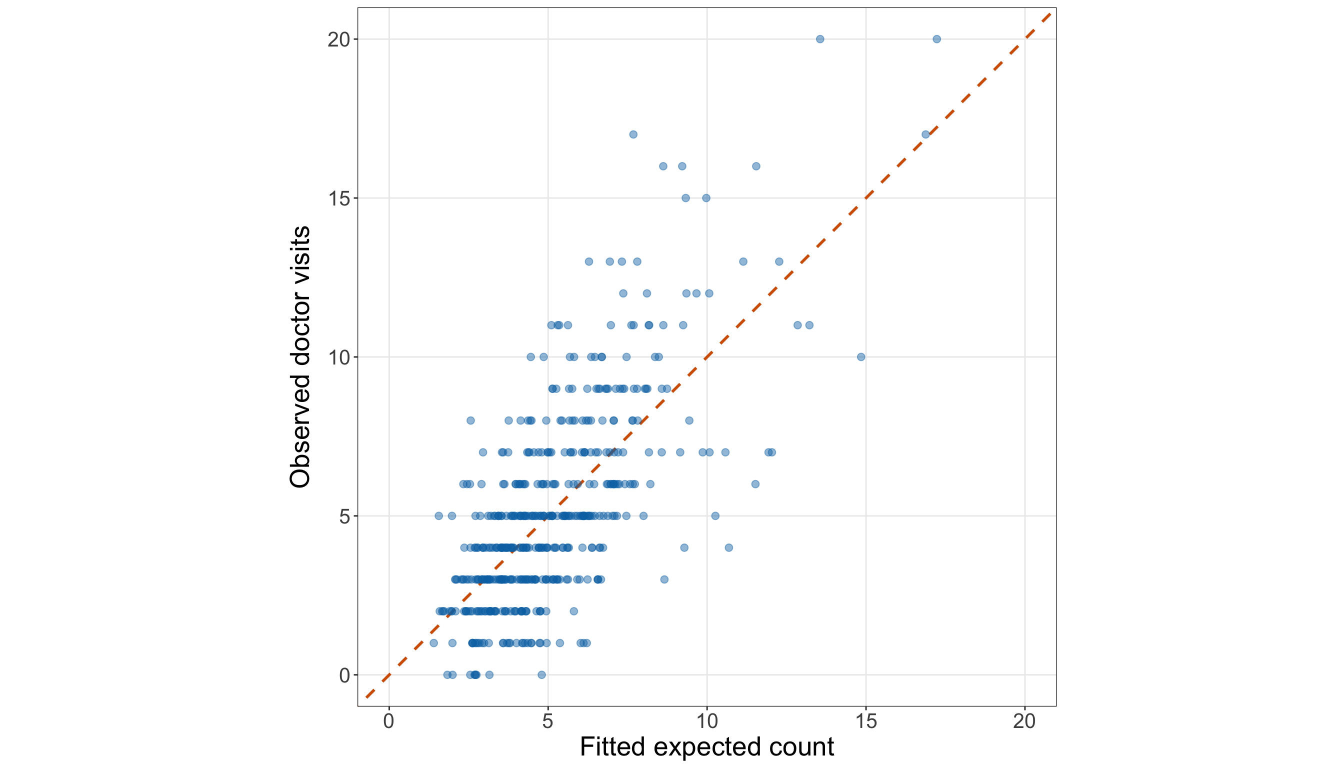
# Common axis limit for the observed-versus-fitted comparison
doctor_extended_observed_fitted_limit = max(
    doctor_extended_poisson_gof_data[
        "doctor_visits"
    ].max(),
    doctor_extended_poisson_gof_data[
        "fitted_expected_count"
    ].max(),
)

# Plotting observed counts against fitted expected counts
(
    doctor_extended_observed_fitted_figure,
    doctor_extended_observed_fitted_axis,
) = plt.subplots(
    figsize=(14, 8)
)

_ = doctor_extended_observed_fitted_axis.plot(
    [0, doctor_extended_observed_fitted_limit],
    [0, doctor_extended_observed_fitted_limit],
    linestyle="--",
    linewidth=1.5,
    color="#D55E00",
)

_ = doctor_extended_observed_fitted_axis.scatter(
    doctor_extended_poisson_gof_data[
        "fitted_expected_count"
    ],
    doctor_extended_poisson_gof_data[
        "doctor_visits"
    ],
    alpha=0.45,
    s=35,
    color="#0072B2",
)

_ = doctor_extended_observed_fitted_axis.set_xlim(
    0,
    doctor_extended_observed_fitted_limit,
)

_ = doctor_extended_observed_fitted_axis.set_ylim(
    0,
    doctor_extended_observed_fitted_limit,
)

_ = doctor_extended_observed_fitted_axis.set_aspect(
    "equal",
    adjustable="box",
)

_ = doctor_extended_observed_fitted_axis.set_xlabel(
    "Fitted expected count",
    fontsize=20,
)

_ = doctor_extended_observed_fitted_axis.set_ylabel(
    "Observed doctor visits",
    fontsize=20,
    labelpad=12,
)

doctor_extended_observed_fitted_axis.tick_params(
    axis="both",
    labelsize=15.5,
)

doctor_extended_observed_fitted_axis.grid(
    True,
    which="major",
    axis="both",
    alpha=0.3,
)

doctor_extended_observed_fitted_axis.grid(
    False,
    which="minor",
)

doctor_extended_observed_fitted_figure.tight_layout()
plt.show()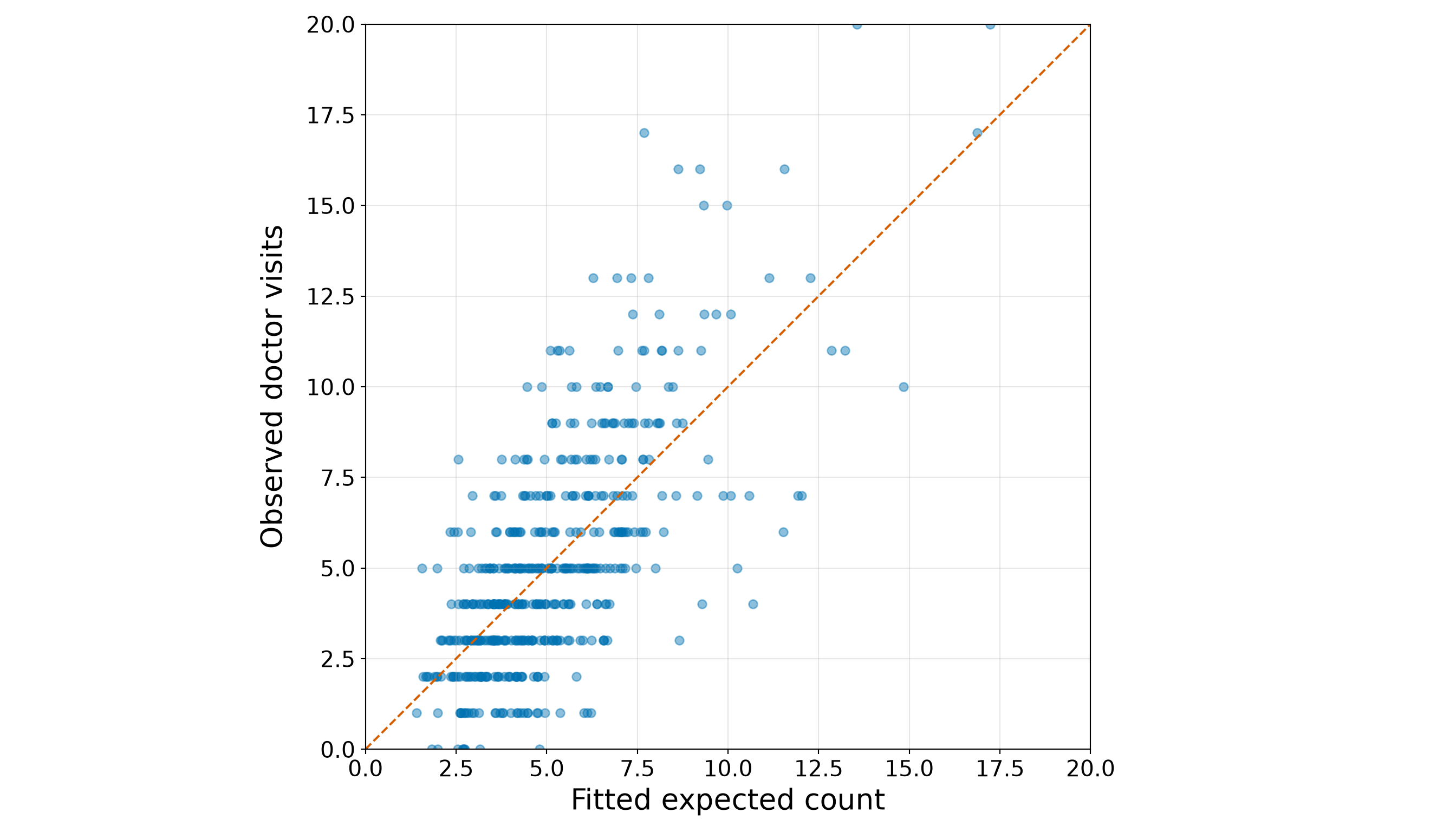
The extended fitted expected counts range from 1.402 to 17.228. This is a wider fitted-mean range than the simple age-only model produced because the extended specification can distinguish individuals of similar ages using income, education, marriage status, urban residence, and insurance.
The points in Figure 10.32 (or Figure 10.33) still do not lie perfectly on the equality line, nor should they: an expected count is not an exact prediction of an individual’s realized count. The relevant question is whether the remaining discrepancies are compatible with the Classical Poisson conditional distribution. We answer that next through formal and graphical goodness-of-fit checks.
Question 10.42 — Rechecking the Extended Model’s Distributional Fit
For the extended training-set model:
- Calculate the Pearson Chi-squared statistic, residual degrees of freedom, dispersion estimate, and one-sided overdispersion \(p\)-value.
- Compare the observed number of zero counts with the fitted expected number of zeros and calculate the approximate one-sided excess-zero \(p\)-value.
- Calculate the residual deviance, residual-deviance ratio, and upper-tail goodness-of-fit \(p\)-value.
- Plot the Pearson residuals against the fitted expected counts and count residuals above \(2\) and below \(-2\).
- Determine whether the extended Classical Poisson model shows evidence of overdispersion, excess zeros, or global lack of fit at the 5% significance level.
Answer 10.42
Click here to reveal the answer!
The mathematics of these checks is unchanged from Question 10.38. Therefore, in Table 10.112, we calculate the three diagnostics together, while retaining their distinct interpretations:
- the Pearson check targets remaining conditional variability relative to the Poisson variance;
- the zero-count check targets more observed zeros than the fitted model expects; and
- the residual deviance provides a global comparison with the saturated benchmark.
# Pearson-dispersion check
doctor_extended_pearson_chi_squared <- sum(
  residuals(
    doctor_extended_poisson_model,
    type = "pearson"
  )^2
)

doctor_extended_pearson_df <- df.residual(
  doctor_extended_poisson_model
)

doctor_extended_pearson_dispersion <-
  doctor_extended_pearson_chi_squared /
  doctor_extended_pearson_df

doctor_extended_pearson_p_value <- pchisq(
  doctor_extended_pearson_chi_squared,
  df = doctor_extended_pearson_df,
  lower.tail = FALSE
)

# Zero-count check
doctor_extended_observed_zero_count <- sum(
  doctor_extended_poisson_gof_data$doctor_visits == 0
)

doctor_extended_expected_zero_count <- sum(
  doctor_extended_poisson_gof_data$fitted_zero_probability
)

doctor_extended_zero_count_variance <- sum(
  doctor_extended_poisson_gof_data$fitted_zero_probability *
    (
      1 -
      doctor_extended_poisson_gof_data$fitted_zero_probability
    )
)

doctor_extended_zero_count_z <- (
  doctor_extended_observed_zero_count -
    doctor_extended_expected_zero_count
) / sqrt(doctor_extended_zero_count_variance)

doctor_extended_zero_count_p_value <- pnorm(
  doctor_extended_zero_count_z,
  lower.tail = FALSE
)

# Residual-deviance check
doctor_extended_residual_deviance <- deviance(
  doctor_extended_poisson_model
)

doctor_extended_residual_deviance_df <- df.residual(
  doctor_extended_poisson_model
)

doctor_extended_residual_deviance_ratio <-
  doctor_extended_residual_deviance /
  doctor_extended_residual_deviance_df

doctor_extended_residual_deviance_p_value <- pchisq(
  doctor_extended_residual_deviance,
  df = doctor_extended_residual_deviance_df,
  lower.tail = FALSE
)

# Consolidated summary table
doctor_extended_gof_summary <- tibble(
  diagnostic = c(
    "Pearson",
    "Pearson",
    "Pearson",
    "Pearson",
    "Zero count",
    "Zero count",
    "Zero count",
    "Zero count",
    "Residual deviance",
    "Residual deviance",
    "Residual deviance",
    "Residual deviance"
  ),
  quantity = c(
    "Chi-squared statistic",
    "Residual degrees of freedom",
    "Dispersion estimate",
    "One-sided overdispersion p-value",
    "Observed zero count",
    "Fitted expected zero count",
    "Approximate z-statistic",
    "One-sided excess-zero p-value",
    "Residual deviance",
    "Residual degrees of freedom",
    "Residual deviance / df",
    "Goodness-of-fit p-value"
  ),
  value = c(
    formatC(
      doctor_extended_pearson_chi_squared,
      format = "f",
      digits = 3
    ),
    formatC(
      doctor_extended_pearson_df,
      format = "f",
      digits = 0
    ),
    formatC(
      doctor_extended_pearson_dispersion,
      format = "f",
      digits = 3
    ),
    formatC(
      doctor_extended_pearson_p_value,
      format = "e",
      digits = 2
    ),
    formatC(
      doctor_extended_observed_zero_count,
      format = "f",
      digits = 0
    ),
    formatC(
      doctor_extended_expected_zero_count,
      format = "f",
      digits = 2
    ),
    formatC(
      doctor_extended_zero_count_z,
      format = "f",
      digits = 2
    ),
    formatC(
      doctor_extended_zero_count_p_value,
      format = "e",
      digits = 2
    ),
    formatC(
      doctor_extended_residual_deviance,
      format = "f",
      digits = 3
    ),
    formatC(
      doctor_extended_residual_deviance_df,
      format = "f",
      digits = 0
    ),
    formatC(
      doctor_extended_residual_deviance_ratio,
      format = "f",
      digits = 3
    ),
    formatC(
      doctor_extended_residual_deviance_p_value,
      format = "e",
      digits = 2
    )
  )
)

doctor_extended_gof_summary |>
  rename(
    `Diagnostic` = diagnostic,
    `Quantity` = quantity,
    `Value` = value
  ) |>
  kable(
    align = c("c", "c", "c")
)| Diagnostic | Quantity | Value |
|---|---|---|
| Pearson | Chi-squared statistic | 483.870 |
| Pearson | Residual degrees of freedom | 493 |
| Pearson | Dispersion estimate | 0.981 |
| Pearson | One-sided overdispersion p-value | 6.07e-01 |
| Zero count | Observed zero count | 9 |
| Zero count | Fitted expected zero count | 11.64 |
| Zero count | Approximate z-statistic | -0.80 |
| Zero count | One-sided excess-zero p-value | 7.90e-01 |
| Residual deviance | Residual deviance | 506.345 |
| Residual deviance | Residual degrees of freedom | 493 |
| Residual deviance | Residual deviance / df | 1.027 |
| Residual deviance | Goodness-of-fit p-value | 3.29e-01 |
from scipy import stats

# Pearson-dispersion check
doctor_extended_pearson_chi_squared = np.sum(
    doctor_extended_poisson_model.resid_pearson ** 2
)

doctor_extended_pearson_df = (
    doctor_extended_poisson_model.df_resid
)

doctor_extended_pearson_dispersion = (
    doctor_extended_pearson_chi_squared
    / doctor_extended_pearson_df
)

doctor_extended_pearson_p_value = stats.chi2.sf(
    doctor_extended_pearson_chi_squared,
    doctor_extended_pearson_df,
)

# Zero-count check
doctor_extended_observed_zero_count = (
    doctor_extended_poisson_gof_data[
        "doctor_visits"
    ]
    == 0
).sum()

doctor_extended_expected_zero_count = (
    doctor_extended_poisson_gof_data[
        "fitted_zero_probability"
    ].sum()
)

doctor_extended_zero_count_variance = (
    doctor_extended_poisson_gof_data[
        "fitted_zero_probability"
    ]
    * (
        1
        - doctor_extended_poisson_gof_data[
            "fitted_zero_probability"
        ]
    )
).sum()

doctor_extended_zero_count_z = (
    doctor_extended_observed_zero_count
    - doctor_extended_expected_zero_count
) / np.sqrt(doctor_extended_zero_count_variance)

doctor_extended_zero_count_p_value = stats.norm.sf(
    doctor_extended_zero_count_z
)

# Residual-deviance check
doctor_extended_residual_deviance = (
    doctor_extended_poisson_model.deviance
)

doctor_extended_residual_deviance_df = (
    doctor_extended_poisson_model.df_resid
)

doctor_extended_residual_deviance_ratio = (
    doctor_extended_residual_deviance
    / doctor_extended_residual_deviance_df
)

doctor_extended_residual_deviance_p_value = stats.chi2.sf(
    doctor_extended_residual_deviance,
    doctor_extended_residual_deviance_df,
)

# Consolidated summary table
doctor_extended_gof_summary = pd.DataFrame(
    {
        "Diagnostic": [
            "Pearson",
            "Pearson",
            "Pearson",
            "Pearson",
            "Zero count",
            "Zero count",
            "Zero count",
            "Zero count",
            "Residual deviance",
            "Residual deviance",
            "Residual deviance",
            "Residual deviance",
        ],
        "Quantity": [
            "Chi-squared statistic",
            "Residual degrees of freedom",
            "Dispersion estimate",
            "One-sided overdispersion p-value",
            "Observed zero count",
            "Fitted expected zero count",
            "Approximate z-statistic",
            "One-sided excess-zero p-value",
            "Residual deviance",
            "Residual degrees of freedom",
            "Residual deviance / df",
            "Goodness-of-fit p-value",
        ],
        "Value": [
            f"{doctor_extended_pearson_chi_squared:.3f}",
            f"{doctor_extended_pearson_df:.0f}",
            f"{doctor_extended_pearson_dispersion:.3f}",
            f"{doctor_extended_pearson_p_value:.2e}",
            f"{doctor_extended_observed_zero_count:.0f}",
            f"{doctor_extended_expected_zero_count:.2f}",
            f"{doctor_extended_zero_count_z:.2f}",
            f"{doctor_extended_zero_count_p_value:.2e}",
            f"{doctor_extended_residual_deviance:.3f}",
            f"{doctor_extended_residual_deviance_df:.0f}",
            f"{doctor_extended_residual_deviance_ratio:.3f}",
            f"{doctor_extended_residual_deviance_p_value:.2e}",
        ],
    }
)

classical_poisson_exercise_doctor_extended_gof_py_html = (
    doctor_extended_gof_summary.to_html(
        index=False,
        border=0,
    )
)| Diagnostic | Quantity | Value |
|---|---|---|
| Pearson | Chi-squared statistic | 483.870 |
| Pearson | Residual degrees of freedom | 493 |
| Pearson | Dispersion estimate | 0.981 |
| Pearson | One-sided overdispersion p-value | 6.07e-01 |
| Zero count | Observed zero count | 9 |
| Zero count | Fitted expected zero count | 11.64 |
| Zero count | Approximate z-statistic | -0.80 |
| Zero count | One-sided excess-zero p-value | 7.90e-01 |
| Residual deviance | Residual deviance | 506.345 |
| Residual deviance | Residual degrees of freedom | 493 |
| Residual deviance | Residual deviance / df | 1.027 |
| Residual deviance | Goodness-of-fit p-value | 3.29e-01 |
For the Pearson check, recall that the hypotheses are the following:
\[ H_0: \phi = 1 \qquad \text{versus} \qquad H_A: \phi > 1. \]
The Pearson dispersion estimate is 0.981, with a one-sided overdispersion \(p\)-value of 6.07e-01. At the 5% significance level, this check does not provide evidence of remaining overdispersion in the extended model.
For the zero-count check, recall that the hypotheses are the following:
\[ \begin{gather} H_0\text{: } \text{the fitted Classical Poisson model adequately describes} \\ \text{the frequency of zero counts}, \\ \text{versus} \\ H_1\text{: } \text{there are more zero counts than the} \\ \text{fitted Classical Poisson model expects}. \end{gather} \]
The training data contain 9 observed zeros, while the extended model expects 11.64 zeros. The one-sided excess-zero \(p\)-value is 7.90e-01. The diagnostic does not provide evidence that the extended model produces too few zeros.
Finally, the hypotheses for the global comparison with the saturated benchmark are the following:
\[ \begin{gather} H_0\text{: } \text{the fitted Classical Poisson model is adequate}, \\ \text{versus} \\ H_1\text{: } \text{the fitted Classical Poisson model is not adequate}. \end{gather} \]
The residual-deviance ratio is 1.027, and the corresponding goodness-of-fit \(p\)-value is 3.29e-01. This global check does not reject the extended Classical Poisson model at the 5% significance level.
Together, these numerical checks assess the distributional fit more directly than the grouped calibration table. We also inspect the Pearson residuals to see how the remaining discrepancies are distributed across fitted expected counts.
# Residual counts used in the interpretation
doctor_extended_large_positive_residuals <- sum(
  doctor_extended_poisson_gof_data$pearson_residual > 2
)

doctor_extended_large_negative_residuals <- sum(
  doctor_extended_poisson_gof_data$pearson_residual < -2
)

doctor_extended_maximum_absolute_residual <- max(
  abs(
    doctor_extended_poisson_gof_data$pearson_residual
  )
)

# Plotting Pearson residuals against fitted expected counts
doctor_extended_pearson_residual_plot <- ggplot(
  doctor_extended_poisson_gof_data,
  aes(
    x = fitted_expected_count,
    y = pearson_residual
  )
) +
  geom_hline(
    yintercept = 0,
    linewidth = 0.8,
    colour = "grey40"
  ) +
  geom_hline(
    yintercept = c(-2, 2),
    linetype = "dashed",
    linewidth = 0.8,
    colour = "#D55E00"
  ) +
  geom_point(
    alpha = 0.60,
    size = 2.3,
    colour = "#0072B2"
  ) +
  theme_bw() +
  theme(
    axis.text = element_text(size = 15.5),
    axis.title.x = element_text(size = 20),
    axis.title.y = element_text(
      size = 20,
      vjust = 0.5,
      margin = margin(r = 12)
    ),
    panel.grid.minor = element_blank()
  ) +
  labs(
    x = "Fitted expected count",
    y = "Pearson residual"
  )

doctor_extended_pearson_residual_plot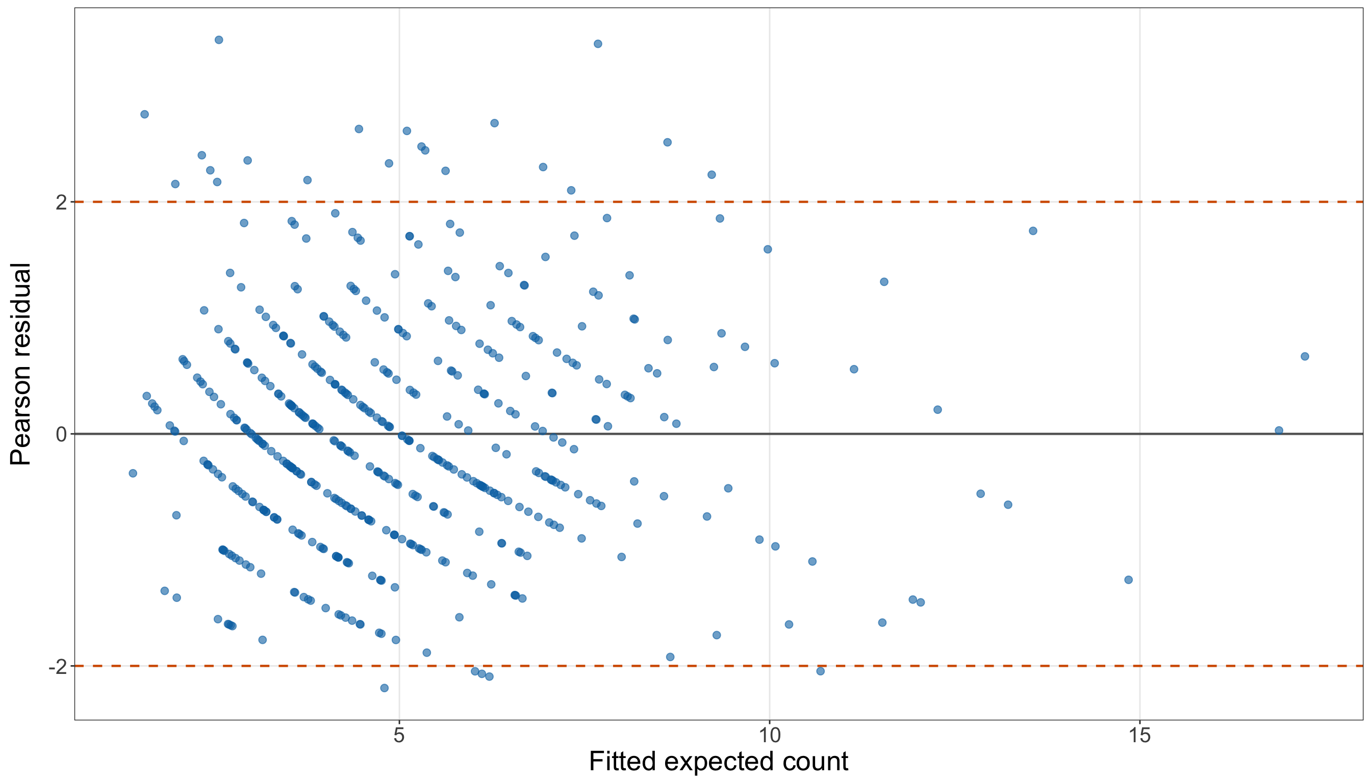
# Residual counts used in the interpretation
doctor_extended_large_positive_residuals = (
    doctor_extended_poisson_gof_data[
        "pearson_residual"
    ]
    > 2
).sum()

doctor_extended_large_negative_residuals = (
    doctor_extended_poisson_gof_data[
        "pearson_residual"
    ]
    < -2
).sum()

doctor_extended_maximum_absolute_residual = np.abs(
    doctor_extended_poisson_gof_data[
        "pearson_residual"
    ]
).max()

# Plotting Pearson residuals against fitted expected counts
(
    doctor_extended_pearson_residual_figure,
    doctor_extended_pearson_residual_axis,
) = plt.subplots(
    figsize=(14, 8)
)

_ = doctor_extended_pearson_residual_axis.axhline(
    0,
    linewidth=0.8,
    color="grey",
)

_ = doctor_extended_pearson_residual_axis.axhline(
    2,
    linestyle="--",
    linewidth=0.8,
    color="#D55E00",
)

_ = doctor_extended_pearson_residual_axis.axhline(
    -2,
    linestyle="--",
    linewidth=0.8,
    color="#D55E00",
)

_ = doctor_extended_pearson_residual_axis.scatter(
    doctor_extended_poisson_gof_data[
        "fitted_expected_count"
    ],
    doctor_extended_poisson_gof_data[
        "pearson_residual"
    ],
    alpha=0.60,
    s=35,
    color="#0072B2",
)

_ = doctor_extended_pearson_residual_axis.set_xlabel(
    "Fitted expected count",
    fontsize=20,
)

_ = doctor_extended_pearson_residual_axis.set_ylabel(
    "Pearson residual",
    fontsize=20,
    labelpad=12,
)

doctor_extended_pearson_residual_axis.tick_params(
    axis="both",
    labelsize=15.5,
)

doctor_extended_pearson_residual_axis.grid(
    True,
    which="major",
    axis="both",
    alpha=0.3,
)

doctor_extended_pearson_residual_axis.grid(
    False,
    which="minor",
)

doctor_extended_pearson_residual_figure.tight_layout()
plt.show()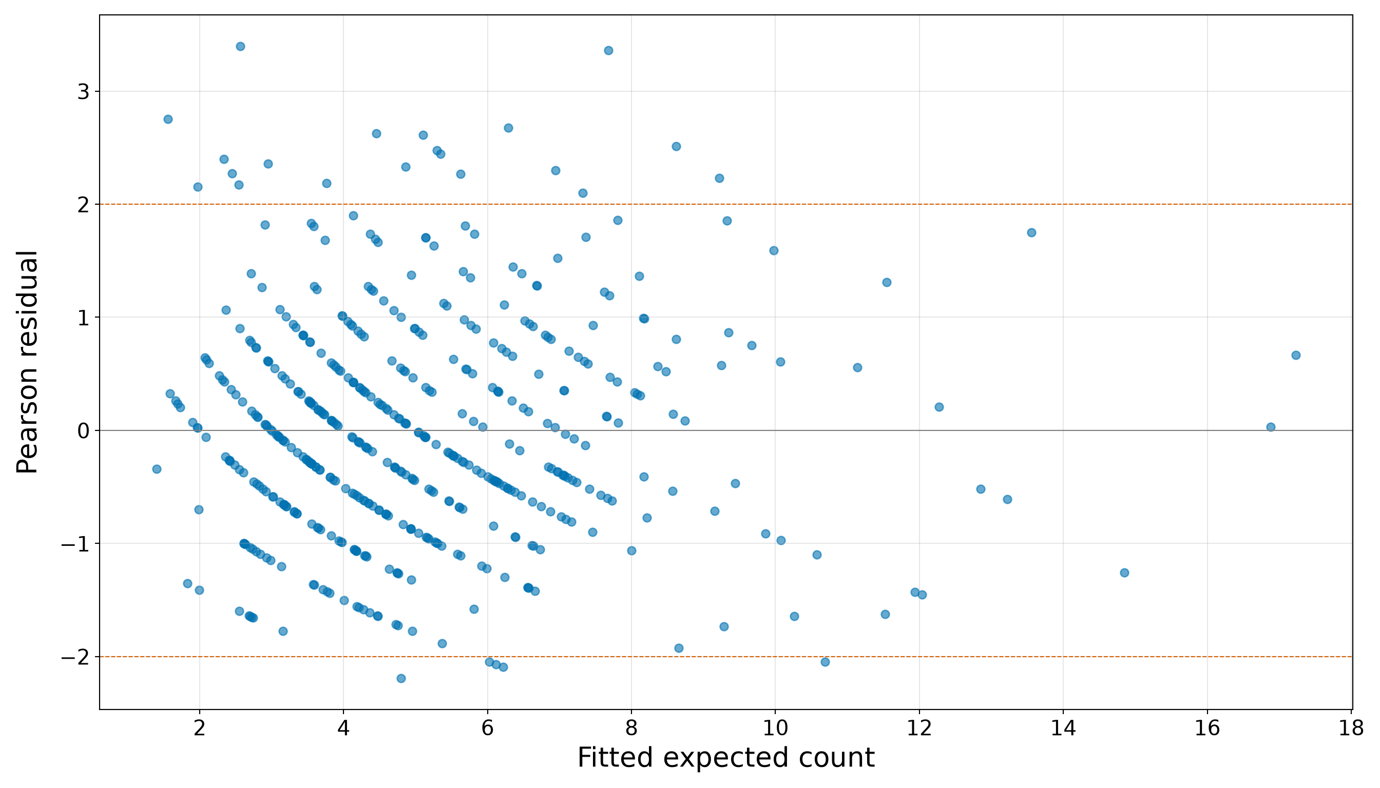
The residual plot in Figure 10.34 (or Figure 10.35) contains 20 Pearson residuals above \(2\) and 5 below \(-2\). The largest absolute Pearson residual is 3.396. These observations deserve attention because the model fits them less closely than most of the training sample. Nevertheless, a finite sample can contain some large residuals even when the global checks do not reject the fitted distribution.
Therefore, the residual plot should be interpreted with the numerical diagnostics rather than replacing them. A visible collection of individual discrepancies is not equivalent to systematic overdispersion, excess zeros, or a globally excessive residual deviance.
Question 10.43 — Deciding Whether the Extended Model Can Proceed to Results
Bring together the model-development evidence from Questions 10.40 to 10.42:
- Compare the simple and extended models’ Pearson dispersion estimates and residual-deviance ratios.
- Compare their zero-count diagnostics.
- State whether the extended model shows evidence of overdispersion, excess zeros, or global lack of fit at the 5% significance level.
- Explain whether the selected extended specification can proceed to the results stage.
- State precisely how the untouched testing set will be used for the inferential and predictive inquiries.
Answer 10.43
Click here to reveal the answer!
Table 10.114 summarizes the diagnostic transition from the simple age-only model to the extended model.
| Diagnostic | Simple age-only model | Extended model | Development-stage interpretation |
|---|---|---|---|
| Pearson dispersion estimate | 1.318 | 0.981 | The remaining conditional variability is substantially closer to the Classical Poisson benchmark after the additional regressors are included. |
| Pearson overdispersion \(p\)-value | 2.31e-06 | 6.07e-01 | The extended model no longer shows statistically detectable overdispersion at the 5% significance level. |
| Observed versus fitted expected zeros | 9 versus 8.37 | 9 versus 11.64 | The extended model does not show evidence of excess zeros. |
| One-sided excess-zero \(p\)-value | 4.12e-01 | 7.90e-01 | The zero-count conclusion is kept separate from the broader dispersion and deviance conclusions. |
| Residual deviance / df | 1.356 | 1.027 | The global discrepancy relative to the saturated model is much closer to its reference scale in the extended specification. |
| Residual-deviance \(p\)-value | 1.80e-07 | 3.29e-01 | The global check does not reject the extended model at the 5% significance level. |
| Pearson residuals outside \([-2,2]\) | 43 | 25 | Some individual discrepancies remain and should be acknowledged, even when the global distributional checks are acceptable. |
At the 5% significance level, none of the three principal checks provides evidence against the extended Classical Poisson model: the Pearson check does not identify overdispersion, the one-sided zero-count check does not identify excess zeros, and the residual-deviance check does not identify global lack of fit.
This comparison is consistent with much of the simple model’s lack of fit arising from an underspecified conditional mean. Once income, education, marriage status, urban residence, and insurance are added alongside age, the remaining variability is much more compatible with the Classical Poisson assumptions. This does not prove that the extended model is the true data-generating mechanism, nor does it eliminate every individual residual discrepancy. It means that the selected model has passed the prespecified training-set checks well enough to proceed in this case-study workflow.
The testing set has still not been used for EDA, model choice, coefficient interpretation, or goodness-of-fit decisions. In the next results stage, it will be used in two deliberately different ways:
-
Inferential inquiry: refit the selected extended specification on
doctor_testing_dataand use that independent fit for the final coefficient estimates, model-based standard errors, Wald tests, confidence intervals, and adjusted conclusions on variable association. -
Predictive inquiry: retain the extended model fitted on
doctor_training_data, generate fitted expected counts fordoctor_testing_data, and assess those held-out predictions against the observed testing counts using the selected prediction metrics and baseline comparison.
Thus, the model specification is now fixed before either final results workflow begins.
Results
The model-development stage is now complete. The simple age-only model was useful for identifying a clear age pattern, but its goodness-of-fit checks showed that the conditional mean was underspecified. After income, education, marriage status, urban residence, and insurance were added, the extended Classical Poisson model passed the prespecified training-set checks well enough to proceed. Most importantly, the model specification is now fixed. Hence, we will not add, remove, or transform regressors after examining the testing-set results.
The two original inquiries now require two different uses of the untouched testing set, as summarized in Table 10.115.
| Inquiry | Model and data used in the results stage | Primary outputs |
|---|---|---|
| Inferential | Refit the selected extended specification on doctor_testing_data. |
Coefficient estimates, model-based standard errors, expected-count ratios, 95% confidence intervals, Wald tests, and adjusted association statements. |
| Predictive | Retain the extended model fitted on doctor_training_data and predict the responses in doctor_testing_data without refitting. |
Held-out predicted expected counts, MAE, RMSE, mean Poisson deviance, an observed-versus-predicted plot, and comparison with the training-mean baseline. |
This distinction is essential given the following:
- For inference, the testing observations provide an independent sample on which to estimate the already selected model specification.
- For prediction, the testing responses must remain unknown to the fitted model: the training-fitted model produces the predictions, and only then are those predictions compared with the observed testing counts.
Heads-up on using the same testing set for two results workflows!
The testing set supports both final analyses, but the two outputs should not be treated as independent replications of the evidence.
- The inferential refit uses the testing responses to estimate the selected model’s coefficients and uncertainty.
- The predictive assessment uses the same testing responses only after the training-fitted model has generated its predictions.
Neither result should be used to revise the model and then be reported again on the same testing observations. Any model revision motivated by these final results would require a new validation sample or another explicitly designed validation procedure.
Question 10.44 — Producing the Final Inferential Results
For the inferential inquiry, use only doctor_testing_data and the extended specification selected during model development:
- Create
income_1000by expressing annual income in thousands of dollars. - Refit the extended Classical Poisson regression using
age,income_1000,education_years,married,urban, andinsurance. - Report the coefficient estimates, model-based standard errors, Wald statistics, and two-sided Wald-test \(p\)-values on the log expected-count scale.
- Exponentiate the non-intercept coefficients and construct approximate 95% Wald confidence intervals on the expected-count ratio scale.
- At the 5% significance level, identify which regressors provide evidence of an adjusted association with the expected number of doctor visits.
- Answer the inferential inquiry while distinguishing association from causation and failure to reject from evidence of no association.
Answer 10.44
Click here to reveal the answer!
The selected specification is the same one developed and checked using the training data. For individual \(i\) in the testing set, define:
- \(x_{i,1}\) as age in years;
- \(x_{i,2}\) as annual income in thousands of dollars;
- \(x_{i,3}\) as years of education;
- \(x_{i,4}=1\) for a married individual and \(0\) for a not-married individual;
- \(x_{i,5}=1\) for an urban resident and \(0\) for a non-urban resident; and
- \(x_{i,6}=1\) for an insured individual and \(0\) for an uninsured individual.
The final inferential refit therefore assumes
\[ Y_i \mid x_{i,1},x_{i,2},\ldots,x_{i,6} \sim \operatorname{Poisson}(\mu_i), \]
with
\[ \begin{align*} \log(\mu_i) =& \beta_0 + \beta_1x_{i,1} + \beta_2x_{i,2} + \beta_3x_{i,3} + \\ & \beta_4x_{i,4} + \beta_5x_{i,5} + \beta_6x_{i,6}. \end{align*} \tag{10.23}\]
The reference categories remain Not married, Non-urban, and Uninsured. The specification in Equation 10.23 was fixed before the testing responses were used.
We first report the testing-set refit on the log expected-count scale. This is the scale on which the model is fitted and on which each Wald statistic is calculated:
\[ Z_j = \frac{\widehat{\beta}_j} {\operatorname{SE}(\widehat{\beta}_j)}. \]
The corresponding two-sided test compares
\[ H_0\text{: }\beta_j=0 \qquad\text{versus}\qquad H_1\text{: }\beta_j\neq 0. \]
# Preparing the independent inferential dataset
doctor_final_inference_data <- doctor_testing_data |>
  mutate(
    income_1000 = income / 1000
  )

# Refitting the selected specification on the testing data
doctor_final_inference_model <- glm(
  formula = doctor_visits ~
    age +
    income_1000 +
    education_years +
    married +
    urban +
    insurance,
  family = poisson(link = "log"),
  data = doctor_final_inference_data
)

# Constructing coefficient-level inferential quantities
doctor_final_inference_summary <- tidy(
  doctor_final_inference_model
) |>
  mutate(
    term_label = case_when(
      term == "(Intercept)" ~ "Intercept",
      term == "age" ~ "Age",
      term == "income_1000" ~ "Income (per $1,000)",
      term == "education_years" ~ "Education (years)",
      term == "marriedMarried" ~ "Married vs not married",
      term == "urbanUrban" ~ "Urban vs non-urban",
      term == "insuranceInsured" ~ "Insured vs uninsured",
      TRUE ~ term
    ),
    term_order = case_when(
      term == "(Intercept)" ~ 0,
      term == "age" ~ 1,
      term == "income_1000" ~ 2,
      term == "education_years" ~ 3,
      term == "marriedMarried" ~ 4,
      term == "urbanUrban" ~ 5,
      term == "insuranceInsured" ~ 6,
      TRUE ~ 99
    ),
    lower_95_log = estimate - qnorm(0.975) * std.error,
    upper_95_log = estimate + qnorm(0.975) * std.error,
    expected_count_ratio = exp(estimate),
    lower_95_ratio = exp(lower_95_log),
    upper_95_ratio = exp(upper_95_log),
    percent_change = 100 * (expected_count_ratio - 1),
    wald_decision = case_when(
      term == "(Intercept)" ~ "Not used for the association inquiry",
      p.value < 0.05 ~ "Reject H0 at 5%",
      TRUE ~ "Fail to reject H0 at 5%"
    )
  ) |>
  arrange(term_order)

# Saving rows used in the written interpretation
doctor_final_age_result <- doctor_final_inference_summary |>
  filter(term == "age")

doctor_final_income_result <- doctor_final_inference_summary |>
  filter(term == "income_1000")

doctor_final_education_result <- doctor_final_inference_summary |>
  filter(term == "education_years")

doctor_final_married_result <- doctor_final_inference_summary |>
  filter(term == "marriedMarried")

doctor_final_urban_result <- doctor_final_inference_summary |>
  filter(term == "urbanUrban")

doctor_final_insurance_result <- doctor_final_inference_summary |>
  filter(term == "insuranceInsured")

doctor_final_significant_terms <- doctor_final_inference_summary |>
  filter(
    term != "(Intercept)",
    p.value < 0.05
  ) |>
  pull(term_label)

doctor_final_significant_terms_text <- if (
  length(doctor_final_significant_terms) == 0
) {
  "none of the six regressors"
} else if (
  length(doctor_final_significant_terms) == 1
) {
  doctor_final_significant_terms
} else {
  paste(
    paste(
      doctor_final_significant_terms[
        -length(doctor_final_significant_terms)
      ],
      collapse = ", "
    ),
    doctor_final_significant_terms[
      length(doctor_final_significant_terms)
    ],
    sep = " and "
  )
}

# Formatting only for the displayed log-scale table
doctor_final_inference_log_display <-
  doctor_final_inference_summary |>
  transmute(
    `Term` = term_label,
    `Log-scale estimate` = formatC(
      estimate,
      format = "f",
      digits = 3
    ),
    `Model-based standard error` = formatC(
      std.error,
      format = "f",
      digits = 3
    ),
    `Wald statistic` = formatC(
      statistic,
      format = "f",
      digits = 3
    ),
    `p-value` = format.pval(
      p.value,
      digits = 3,
      eps = 0.001
    )
  )

doctor_final_inference_log_display |>
  kable(
    align = c("c", "c", "c", "c", "c")
)| Term | Log-scale estimate | Model-based standard error | Wald statistic | p-value |
|---|---|---|---|---|
| Intercept | 0.028 | 0.157 | 0.176 | 0.86060 |
| Age | 0.028 | 0.002 | 14.172 | < 0.001 |
| Income (per $1,000) | -0.011 | 0.001 | -8.314 | < 0.001 |
| Education (years) | 0.059 | 0.006 | 9.175 | < 0.001 |
| Married vs not married | 0.097 | 0.040 | 2.439 | 0.01472 |
| Urban vs non-urban | 0.175 | 0.045 | 3.868 | < 0.001 |
| Insured vs uninsured | 0.116 | 0.040 | 2.905 | 0.00367 |
# Preparing the independent inferential dataset
doctor_final_inference_data = doctor_testing_data.copy()

doctor_final_inference_data["income_1000"] = (
    doctor_final_inference_data["income"]
    / 1000
)

# Restoring the intended category order explicitly
doctor_final_inference_data["married"] = pd.Categorical(
    doctor_final_inference_data["married"],
    categories=[
        "Not married",
        "Married",
    ],
)

doctor_final_inference_data["urban"] = pd.Categorical(
    doctor_final_inference_data["urban"],
    categories=[
        "Non-urban",
        "Urban",
    ],
)

doctor_final_inference_data["insurance"] = pd.Categorical(
    doctor_final_inference_data["insurance"],
    categories=[
        "Uninsured",
        "Insured",
    ],
)

# Refitting the selected specification on the testing data
doctor_final_inference_model = smf.glm(
    formula=(
        "doctor_visits ~ age + income_1000 "
        "+ education_years "
        "+ C(married, Treatment(reference='Not married')) "
        "+ C(urban, Treatment(reference='Non-urban')) "
        "+ C(insurance, Treatment(reference='Uninsured'))"
    ),
    data=doctor_final_inference_data,
    family=sm.families.Poisson(),
).fit()

# Defining labels and a common display order
doctor_final_term_labels = {
    "Intercept": "Intercept",
    "age": "Age",
    "income_1000": "Income (per $1,000)",
    "education_years": "Education (years)",
    (
        "C(married, Treatment(reference='Not married'))"
        "[T.Married]"
    ): "Married vs not married",
    (
        "C(urban, Treatment(reference='Non-urban'))"
        "[T.Urban]"
    ): "Urban vs non-urban",
    (
        "C(insurance, Treatment(reference='Uninsured'))"
        "[T.Insured]"
    ): "Insured vs uninsured",
}

doctor_final_term_order = list(
    doctor_final_term_labels.keys()
)

# Constructing coefficient-level inferential quantities
doctor_final_inference_summary = pd.DataFrame(
    {
        "Raw term": doctor_final_inference_model.params.index,
        "Log-scale estimate": doctor_final_inference_model.params.values,
        "Model-based standard error": doctor_final_inference_model.bse.values,
        "Wald statistic": doctor_final_inference_model.tvalues.values,
        "p-value": doctor_final_inference_model.pvalues.values,
    }
)

doctor_final_inference_summary["Term"] = (
    doctor_final_inference_summary["Raw term"]
    .map(doctor_final_term_labels)
)

doctor_final_inference_summary["Term order"] = (
    doctor_final_inference_summary["Raw term"]
    .map(
        {
            term: position
            for position, term in enumerate(
                doctor_final_term_order
            )
        }
    )
)

doctor_final_inference_summary["Lower 95% CI on log scale"] = (
    doctor_final_inference_summary["Log-scale estimate"]
    - stats.norm.ppf(0.975)
    * doctor_final_inference_summary[
        "Model-based standard error"
    ]
)

doctor_final_inference_summary["Upper 95% CI on log scale"] = (
    doctor_final_inference_summary["Log-scale estimate"]
    + stats.norm.ppf(0.975)
    * doctor_final_inference_summary[
        "Model-based standard error"
    ]
)

doctor_final_inference_summary["Expected-count ratio"] = np.exp(
    doctor_final_inference_summary["Log-scale estimate"]
)

doctor_final_inference_summary["Lower 95% CI for ratio"] = np.exp(
    doctor_final_inference_summary[
        "Lower 95% CI on log scale"
    ]
)

doctor_final_inference_summary["Upper 95% CI for ratio"] = np.exp(
    doctor_final_inference_summary[
        "Upper 95% CI on log scale"
    ]
)

doctor_final_inference_summary["Percent change"] = (
    100
    * (
        doctor_final_inference_summary[
            "Expected-count ratio"
        ]
        - 1
    )
)

doctor_final_inference_summary["Wald decision"] = np.where(
    doctor_final_inference_summary["Raw term"] == "Intercept",
    "Not used for the association inquiry",
    np.where(
        doctor_final_inference_summary["p-value"] < 0.05,
        "Reject H0 at 5%",
        "Fail to reject H0 at 5%",
    ),
)

doctor_final_inference_summary = (
    doctor_final_inference_summary
    .sort_values("Term order")
    .reset_index(drop=True)
)

# Formatting only for the displayed log-scale table
doctor_final_inference_log_display = (
    doctor_final_inference_summary[
        [
            "Term",
            "Log-scale estimate",
            "Model-based standard error",
            "Wald statistic",
            "p-value",
        ]
    ]
    .copy()
)

for column in [
    "Log-scale estimate",
    "Model-based standard error",
    "Wald statistic",
]:
    doctor_final_inference_log_display[column] = (
        doctor_final_inference_log_display[column]
        .map(lambda value: f"{value:.3f}")
    )

doctor_final_inference_log_display["p-value"] = (
    doctor_final_inference_log_display["p-value"]
    .map(
        lambda value: (
            "<0.001"
            if value < 0.001
            else f"{value:.3f}"
        )
    )
)

classical_poisson_exercise_doctor_final_inference_log_py_html = (
    doctor_final_inference_log_display.to_html(
        index=False,
        border=0,
    )
)| Term | Log-scale estimate | Model-based standard error | Wald statistic | p-value |
|---|---|---|---|---|
| Intercept | 0.028 | 0.157 | 0.176 | 0.861 |
| Age | 0.028 | 0.002 | 14.172 | <0.001 |
| Income (per $1,000) | -0.011 | 0.001 | -8.314 | <0.001 |
| Education (years) | 0.059 | 0.006 | 9.175 | <0.001 |
| Married vs not married | 0.097 | 0.040 | 2.439 | 0.015 |
| Urban vs non-urban | 0.175 | 0.045 | 3.868 | <0.001 |
| Insured vs uninsured | 0.116 | 0.040 | 2.905 | 0.004 |
The coefficient table in Table 10.116 reports the final refit on the model’s estimation scale. The model-based standard errors rely on the Classical Poisson conditional mean-variance assumption. In this workflow, the earlier training-set diagnostics did not identify remaining overdispersion, excess zeros, or global lack of fit in the extended specification at the 5% significance level. That diagnostic evidence supports proceeding with the Classical Poisson standard errors, although it does not prove that the distributional assumptions are exactly true.
For substantive interpretation, we exponentiate each non-intercept coefficient. An exponentiated coefficient of \(1\) represents no multiplicative difference in the expected count. A value above \(1\) represents a larger expected count, and a value below \(1\) represents a smaller expected count, holding all other regressors fixed. The null hypothesis \(H_0\text{: }\beta_j=0\) is equivalent to \(H_0\text{: }\exp(\beta_j)=1\).
doctor_final_inference_ratio_display <-
  doctor_final_inference_summary |>
  filter(term != "(Intercept)") |>
  transmute(
    `Regressor comparison` = term_label,
    `Expected-count ratio` = formatC(
      expected_count_ratio,
      format = "f",
      digits = 3
    ),
    `Lower 95% CI` = formatC(
      lower_95_ratio,
      format = "f",
      digits = 3
    ),
    `Upper 95% CI` = formatC(
      upper_95_ratio,
      format = "f",
      digits = 3
    ),
    `Percent change` = paste0(
      formatC(
        percent_change,
        format = "f",
        digits = 1
      ),
      "%"
    ),
    `p-value` = format.pval(
      p.value,
      digits = 3,
      eps = 0.001
    ),
    `Wald decision` = wald_decision
  )

doctor_final_inference_ratio_display |>
  kable(
    align = c("c", "c", "c", "c", "c", "c", "c")
)| Regressor comparison | Expected-count ratio | Lower 95% CI | Upper 95% CI | Percent change | p-value | Wald decision |
|---|---|---|---|---|---|---|
| Age | 1.029 | 1.025 | 1.033 | 2.9% | < 0.001 | Reject H0 at 5% |
| Income (per $1,000) | 0.989 | 0.986 | 0.991 | -1.1% | < 0.001 | Reject H0 at 5% |
| Education (years) | 1.061 | 1.047 | 1.074 | 6.1% | < 0.001 | Reject H0 at 5% |
| Married vs not married | 1.102 | 1.019 | 1.191 | 10.2% | 0.01472 | Reject H0 at 5% |
| Urban vs non-urban | 1.191 | 1.090 | 1.301 | 19.1% | < 0.001 | Reject H0 at 5% |
| Insured vs uninsured | 1.123 | 1.038 | 1.214 | 12.3% | 0.00367 | Reject H0 at 5% |
doctor_final_inference_ratio_display = (
    doctor_final_inference_summary.loc[
        doctor_final_inference_summary["Raw term"]
        != "Intercept",
        [
            "Term",
            "Expected-count ratio",
            "Lower 95% CI for ratio",
            "Upper 95% CI for ratio",
            "Percent change",
            "p-value",
            "Wald decision",
        ],
    ]
    .copy()
    .rename(
        columns={
            "Term": "Regressor comparison",
            "Lower 95% CI for ratio": "Lower 95% CI",
            "Upper 95% CI for ratio": "Upper 95% CI",
        }
    )
)

for column in [
    "Expected-count ratio",
    "Lower 95% CI",
    "Upper 95% CI",
]:
    doctor_final_inference_ratio_display[column] = (
        doctor_final_inference_ratio_display[column]
        .map(lambda value: f"{value:.3f}")
    )

doctor_final_inference_ratio_display["Percent change"] = (
    doctor_final_inference_ratio_display["Percent change"]
    .map(lambda value: f"{value:.1f}%")
)

doctor_final_inference_ratio_display["p-value"] = (
    doctor_final_inference_ratio_display["p-value"]
    .map(
        lambda value: (
            "<0.001"
            if value < 0.001
            else f"{value:.3f}"
        )
    )
)

classical_poisson_exercise_doctor_final_inference_ratios_py_html = (
    doctor_final_inference_ratio_display.to_html(
        index=False,
        border=0,
    )
)| Regressor comparison | Expected-count ratio | Lower 95% CI | Upper 95% CI | Percent change | p-value | Wald decision |
|---|---|---|---|---|---|---|
| Age | 1.029 | 1.025 | 1.033 | 2.9% | <0.001 | Reject H0 at 5% |
| Income (per $1,000) | 0.989 | 0.986 | 0.991 | -1.1% | <0.001 | Reject H0 at 5% |
| Education (years) | 1.061 | 1.047 | 1.074 | 6.1% | <0.001 | Reject H0 at 5% |
| Married vs not married | 1.102 | 1.019 | 1.191 | 10.2% | 0.015 | Reject H0 at 5% |
| Urban vs non-urban | 1.191 | 1.090 | 1.301 | 19.1% | <0.001 | Reject H0 at 5% |
| Insured vs uninsured | 1.123 | 1.038 | 1.214 | 12.3% | 0.004 | Reject H0 at 5% |
The continuous-regressor results in Table 10.118 can be read as follows, holding marriage status, urban residence, insurance status, and the other continuous regressors fixed:
- A one-year increase in age is associated with multiplying the expected annual doctor-visit count by 1.029. Equivalently, this corresponds to an estimated 2.9% increase in the expected count. The approximate 95% confidence interval for the expected-count ratio is (1.025, 1.033), which corresponds to a 95% confidence interval of (2.5%, 3.3%) on the percentage-change scale. The Wald-test \(p\)-value is <0.001.
- A \(\$1{,}000\) increase in annual income is associated with multiplying the expected annual doctor-visit count by 0.989. Equivalently, this corresponds to an estimated 1.1% decrease in the expected count. The approximate 95% confidence interval for the expected-count ratio is (0.986, 0.991), which corresponds to a 95% confidence interval of (-1.4%, -0.9%) on the percentage-change scale. The Wald-test \(p\)-value is <0.001.
- One additional year of education is associated with multiplying the expected annual doctor-visit count by 1.061. Equivalently, this corresponds to an estimated 6.1% increase in the expected count. The approximate 95% confidence interval for the expected-count ratio is (1.047, 1.074), which corresponds to a 95% confidence interval of (4.7%, 7.4%) on the percentage-change scale. The Wald-test \(p\)-value is <0.001.
The categorical-regressor results compare individuals who share the same values of age, income, education, and the remaining categorical regressors:
- Married individuals have an estimated expected annual doctor-visit count that is 1.102 times that of not-married individuals, holding the other regressors fixed. Equivalently, married individuals are estimated to have an expected count that is 10.2% higher than that of not-married individuals. The approximate 95% confidence interval for the expected-count ratio is (1.019, 1.191), which corresponds to a 95% confidence interval of (1.9%, 19.1%) on the percentage-change scale. The Wald-test \(p\)-value is 0.0147.
- Urban residents have an estimated expected annual doctor-visit count that is 1.191 times that of non-urban residents, holding the other regressors fixed. Equivalently, urban residents are estimated to have an expected count that is 19.1% higher than that of non-urban residents. The approximate 95% confidence interval for the expected-count ratio is (1.090, 1.301), which corresponds to a 95% confidence interval of (9.0%, 30.1%) on the percentage-change scale. The Wald-test \(p\)-value is <0.001.
- Insured individuals have an estimated expected annual doctor-visit count that is 1.123 times that of uninsured individuals, holding the other regressors fixed. Equivalently, insured individuals are estimated to have an expected count that is 12.3% higher than that of uninsured individuals. The approximate 95% confidence interval for the expected-count ratio is (1.038, 1.214), which corresponds to a 95% confidence interval of (3.8%, 21.4%) on the percentage-change scale. The Wald-test \(p\)-value is 0.00367.
At the 5% significance level, the coefficient-level Wald tests identify Age, Income (per $1,000), Education (years), Married vs not married, Urban vs non-urban and Insured vs uninsured as providing evidence of adjusted association with the expected annual doctor-visit count. A confidence interval that excludes \(1\) on the expected-count ratio scale gives the same coefficient-level decision as the corresponding two-sided Wald test at the 5% level.
The inferential conclusion must remain appropriately limited. These data are observational, so the coefficient estimates describe conditional associations under the fitted model; they do not establish that changing age, income, education, marriage status, urban residence, or insurance status would cause a change in doctor visits. Likewise, a failure to reject \(H_0\) does not demonstrate that a regressor has no association. It indicates that the testing-set refit does not provide sufficiently strong evidence against an expected-count ratio of \(1\) at the selected significance level.
Question 10.45 — Evaluating Held-Out Predictive Performance
For the predictive inquiry:
-
Keep the extended model fitted on
doctor_training_data; do not refit it on the testing data. - Create
income_1000indoctor_testing_dataand generate a predicted expected doctor-visit count for every testing observation. - Construct a training-mean baseline that predicts the mean training-set doctor-visit count for every testing observation.
- For the extended model and baseline, report the mean error (ME), MAE, RMSE, and mean Poisson deviance.
- Construct an observed-versus-predicted plot for the extended model with an equality reference line.
- Explain whether the demographic and socioeconomic regressors improve held-out prediction beyond the baseline and why the predicted expected counts should not be rounded into exact count predictions.
Answer 10.45
Click here to reveal the answer!
For testing observation \(i\), let \(y_i\) denote the observed annual number of doctor visits and let \(\widehat{\mu}_i\) denote the expected count predicted by the training-fitted extended model. With \(n_{\operatorname{test}}\) testing observations, we use:
\[ \operatorname{ME} = \frac{1}{n_{\operatorname{test}}} \sum_{i=1}^{n_{\operatorname{test}}} (y_i-\widehat{\mu}_i), \]
\[ \operatorname{MAE} = \frac{1}{n_{\operatorname{test}}} \sum_{i=1}^{n_{\operatorname{test}}} \left|y_i-\widehat{\mu}_i\right|, \]
\[ \operatorname{RMSE} = \sqrt{ \frac{1}{n_{\operatorname{test}}} \sum_{i=1}^{n_{\operatorname{test}}} (y_i-\widehat{\mu}_i)^2 }, \]
and
\[ \operatorname{Mean\ Poisson\ deviance} = \frac{2}{n_{\operatorname{test}}} \sum_{i=1}^{n_{\operatorname{test}}} \left[ y_i\log\left(\frac{y_i}{\widehat{\mu}_i}\right) -(y_i-\widehat{\mu}_i) \right], \]
where the term \(y_i\log(y_i/\widehat{\mu}_i)\) is defined to be \(0\) when \(y_i=0\).
The ME is a signed measure: a positive value indicates average underprediction because observed counts tend to exceed predicted expected counts, whereas a negative value indicates average overprediction. MAE and RMSE summarize point-prediction discrepancies, while mean Poisson deviance assesses the predictions on a scale connected to the Poisson likelihood. Smaller MAE, RMSE, and mean Poisson deviance are preferable.
The baseline predicts
\[ \widehat{\mu}_{i,\operatorname{baseline}} = \overline{y}_{\operatorname{train}} \]
for every testing observation. It therefore uses no demographic or socioeconomic information.
# Preparing the held-out testing regressors
doctor_prediction_results <- doctor_testing_data |>
  mutate(
    income_1000 = income / 1000
  )

# Generating expected counts without refitting the training model
doctor_prediction_results <- doctor_prediction_results |>
  mutate(
    predicted_expected_count = predict(
      doctor_extended_poisson_model,
      newdata = doctor_prediction_results,
      type = "response"
    ),
    baseline_predicted_count = mean(
      doctor_training_data$doctor_visits
    )
  )

# Computing the Poisson deviance safely when observed counts equal zero
doctor_poisson_deviance_component <- function(
  observed,
  predicted_mean
) {
  deviance_component <- predicted_mean
  positive_count <- observed > 0

  deviance_component[positive_count] <-
    observed[positive_count] * log(
      observed[positive_count] /
        predicted_mean[positive_count]
    ) -
    observed[positive_count] +
    predicted_mean[positive_count]

  deviance_component
}

# Computing the selected held-out metrics
doctor_prediction_metric_summary <- function(
  observed,
  predicted_mean
) {
  poisson_components <- doctor_poisson_deviance_component(
    observed = observed,
    predicted_mean = predicted_mean
  )

  tibble(
    mean_error = mean(observed - predicted_mean),
    mean_absolute_error = mean(
      abs(observed - predicted_mean)
    ),
    root_mean_squared_error = sqrt(
      mean((observed - predicted_mean)^2)
    ),
    mean_poisson_deviance = 2 * mean(
      poisson_components
    )
  )
}

doctor_extended_prediction_metrics <-
  doctor_prediction_metric_summary(
    observed = doctor_prediction_results$doctor_visits,
    predicted_mean =
      doctor_prediction_results$predicted_expected_count
  ) |>
  mutate(model = "Extended Poisson model")

doctor_baseline_prediction_metrics <-
  doctor_prediction_metric_summary(
    observed = doctor_prediction_results$doctor_visits,
    predicted_mean =
      doctor_prediction_results$baseline_predicted_count
  ) |>
  mutate(model = "Training-mean baseline")

doctor_prediction_metrics <- bind_rows(
  doctor_extended_prediction_metrics,
  doctor_baseline_prediction_metrics
) |>
  select(
    model,
    everything()
  )

# Formatting only for the displayed table
doctor_prediction_metrics |>
  transmute(
    `Model` = model,
    `Mean error` = formatC(
      mean_error,
      format = "f",
      digits = 3
    ),
    `MAE` = formatC(
      mean_absolute_error,
      format = "f",
      digits = 3
    ),
    `RMSE` = formatC(
      root_mean_squared_error,
      format = "f",
      digits = 3
    ),
    `Mean Poisson deviance` = formatC(
      mean_poisson_deviance,
      format = "f",
      digits = 3
    )
  ) |>
  kable(
    align = c("c", "c", "c", "c", "c")
)| Model | Mean error | MAE | RMSE | Mean Poisson deviance |
|---|---|---|---|---|
| Extended Poisson model | 0.015 | 1.710 | 2.212 | 0.996 |
| Training-mean baseline | 0.104 | 2.323 | 3.011 | 1.744 |
# Preparing the held-out testing regressors
doctor_prediction_results = doctor_testing_data.copy()

doctor_prediction_results["income_1000"] = (
    doctor_prediction_results["income"]
    / 1000
)

for regressor, categories in doctor_category_levels.items():
    doctor_prediction_results[regressor] = pd.Categorical(
        doctor_prediction_results[regressor],
        categories=categories,
    )

# Generating expected counts without refitting the training model
doctor_prediction_results["predicted_expected_count"] = (
    doctor_extended_poisson_model.predict(
        doctor_prediction_results
    )
)

doctor_prediction_results["baseline_predicted_count"] = (
    doctor_training_data["doctor_visits"].mean()
)

# Computing the Poisson deviance safely when observed counts equal zero
def doctor_poisson_deviance_component(
    observed,
    predicted_mean,
):
    observed = np.asarray(observed, dtype=float)
    predicted_mean = np.asarray(
        predicted_mean,
        dtype=float,
    )

    deviance_component = predicted_mean.copy()
    positive_count = observed > 0

    deviance_component[positive_count] = (
        observed[positive_count]
        * np.log(
            observed[positive_count]
            / predicted_mean[positive_count]
        )
        - observed[positive_count]
        + predicted_mean[positive_count]
    )

    return deviance_component

# Computing the selected held-out metrics
def doctor_prediction_metric_summary(
    observed,
    predicted_mean,
):
    observed = np.asarray(observed, dtype=float)
    predicted_mean = np.asarray(
        predicted_mean,
        dtype=float,
    )

    poisson_components = doctor_poisson_deviance_component(
        observed=observed,
        predicted_mean=predicted_mean,
    )

    return {
        "Mean error": np.mean(observed - predicted_mean),
        "MAE": np.mean(np.abs(observed - predicted_mean)),
        "RMSE": np.sqrt(
            np.mean((observed - predicted_mean) ** 2)
        ),
        "Mean Poisson deviance": 2 * np.mean(
            poisson_components
        ),
    }

doctor_extended_prediction_metrics = (
    doctor_prediction_metric_summary(
        observed=doctor_prediction_results[
            "doctor_visits"
        ],
        predicted_mean=doctor_prediction_results[
            "predicted_expected_count"
        ],
    )
)

doctor_baseline_prediction_metrics = (
    doctor_prediction_metric_summary(
        observed=doctor_prediction_results[
            "doctor_visits"
        ],
        predicted_mean=doctor_prediction_results[
            "baseline_predicted_count"
        ],
    )
)

doctor_prediction_metrics = pd.DataFrame(
    [
        {
            "Model": "Extended Poisson model",
            **doctor_extended_prediction_metrics,
        },
        {
            "Model": "Training-mean baseline",
            **doctor_baseline_prediction_metrics,
        },
    ]
)

# Formatting only for the displayed table
doctor_prediction_metrics_display = (
    doctor_prediction_metrics.copy()
)

for column in [
    "Mean error",
    "MAE",
    "RMSE",
    "Mean Poisson deviance",
]:
    doctor_prediction_metrics_display[column] = (
        doctor_prediction_metrics_display[column]
        .map(lambda value: f"{value:.3f}")
    )

classical_poisson_exercise_doctor_prediction_metrics_py_html = (
    doctor_prediction_metrics_display.to_html(
        index=False,
        border=0,
    )
)| Model | Mean error | MAE | RMSE | Mean Poisson deviance |
|---|---|---|---|---|
| Extended Poisson model | 0.015 | 1.710 | 2.212 | 0.996 |
| Training-mean baseline | 0.104 | 2.323 | 3.011 | 1.744 |
The table in Table 10.120 is a held-out assessment because doctor_extended_poisson_model was estimated before the testing responses were used. The extended model has a mean error of 0.015. Because the mean error is positive, the model underpredicts the observed counts on average. The signed mean error must not be used alone because positive and negative errors can cancel.
For absolute prediction error, the extended model has an MAE of 1.710, compared with 2.323 for the training-mean baseline. This is 26.4% lower than the baseline value, indicating better performance on this metric. The extended-model RMSE is 2.212, compared with 3.011 for the baseline. This is 26.5% lower than the baseline value, indicating better performance on this metric.
The likelihood-connected comparison gives the extended model a mean Poisson deviance of 0.996, versus 1.744 for the baseline. This is 42.9% lower than the baseline value, indicating better performance on this metric. Overall, the extended model outperforms the training-mean baseline on MAE, RMSE, and mean Poisson deviance.
We now inspect the individual testing observations. The equality line in the following plot represents perfect agreement between an observed count and a predicted expected count. Points above the line have observed counts larger than their fitted expected counts, whereas points below the line have observed counts smaller than their fitted expected counts.
doctor_observed_predicted_plot <- ggplot(
  doctor_prediction_results,
  aes(
    x = predicted_expected_count,
    y = doctor_visits
  )
) +
  geom_abline(
    intercept = 0,
    slope = 1,
    linetype = "dashed",
    linewidth = 0.9,
    colour = "grey40"
  ) +
  geom_point(
    alpha = 0.55,
    size = 2.3,
    colour = "#0072B2"
  ) +
  theme_bw() +
  theme(
    axis.text = element_text(size = 15.5),
    axis.title.x = element_text(size = 20),
    axis.title.y = element_text(
      size = 20,
      vjust = 0.5,
      margin = margin(r = 12)
    ),
    panel.grid.minor = element_blank()
  ) +
  labs(
    x = "Predicted expected doctor visits",
    y = "Observed doctor visits"
  )

doctor_observed_predicted_plot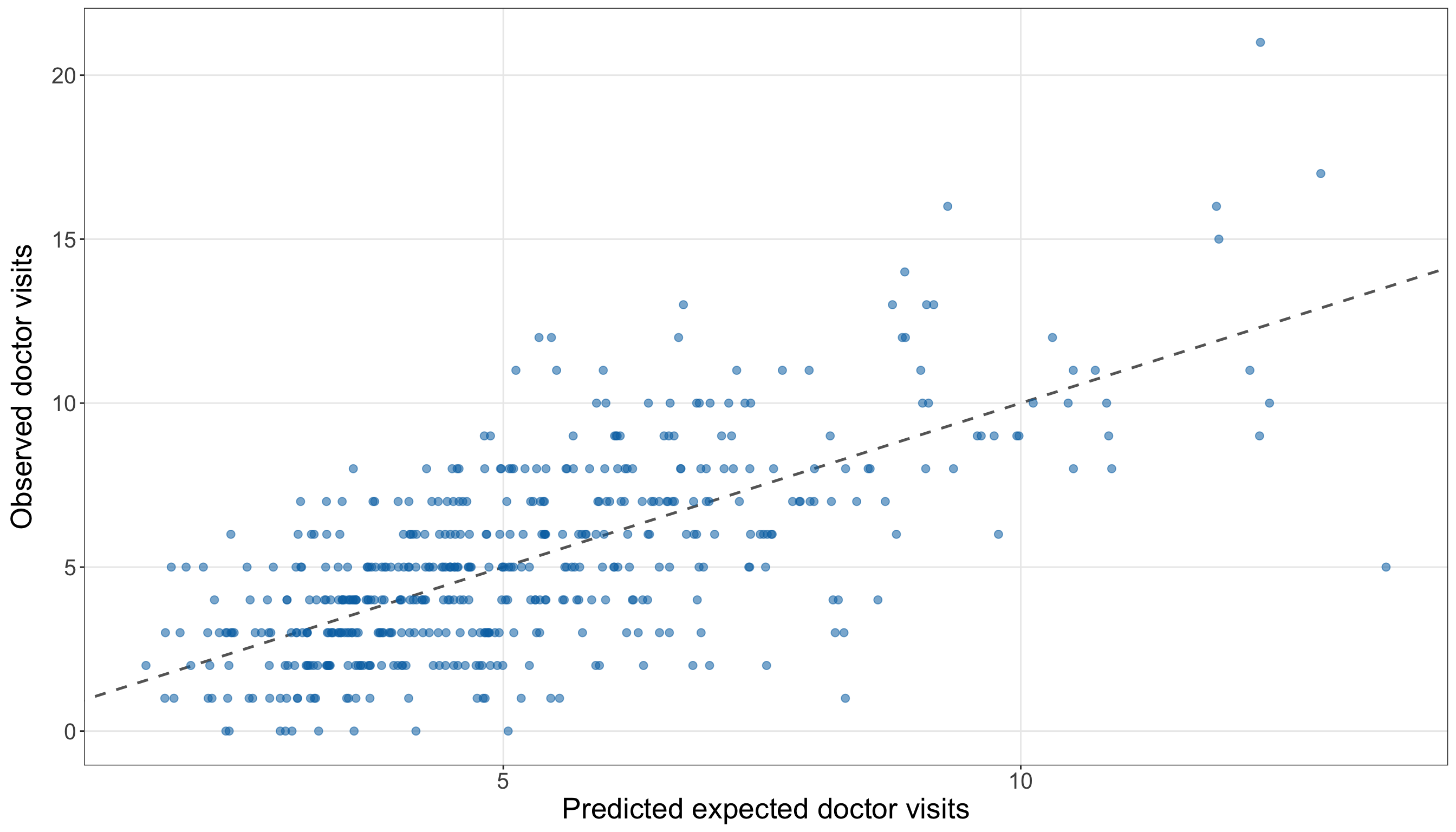
(
    doctor_observed_predicted_figure,
    doctor_observed_predicted_axis,
) = plt.subplots(
    figsize=(14, 8)
)

maximum_doctor_plot_value = max(
    doctor_prediction_results[
        "predicted_expected_count"
    ].max(),
    doctor_prediction_results[
        "doctor_visits"
    ].max(),
)

_ = doctor_observed_predicted_axis.plot(
    [0, maximum_doctor_plot_value],
    [0, maximum_doctor_plot_value],
    linestyle="--",
    linewidth=0.9,
    color="grey",
)

_ = doctor_observed_predicted_axis.scatter(
    doctor_prediction_results[
        "predicted_expected_count"
    ],
    doctor_prediction_results["doctor_visits"],
    alpha=0.55,
    s=35,
    color="#0072B2",
)

_ = doctor_observed_predicted_axis.set_xlabel(
    "Predicted expected doctor visits",
    fontsize=20,
)

_ = doctor_observed_predicted_axis.set_ylabel(
    "Observed doctor visits",
    fontsize=20,
    labelpad=12,
)

doctor_observed_predicted_axis.tick_params(
    axis="both",
    labelsize=15.5,
)

doctor_observed_predicted_axis.grid(
    True,
    which="major",
    axis="both",
    alpha=0.3,
)

doctor_observed_predicted_axis.grid(
    False,
    which="minor",
)

doctor_observed_predicted_figure.tight_layout()
plt.show()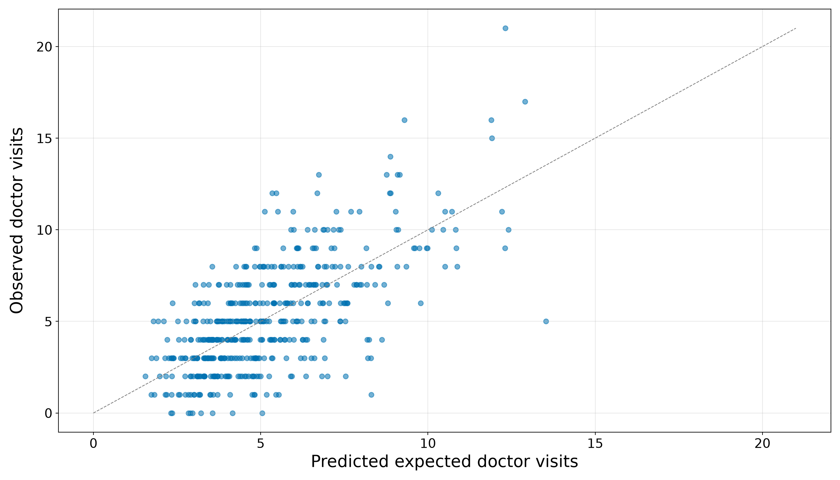
The scatter around the equality line in Figure 10.36 (or Figure 10.37) should not be interpreted as evidence that fractional predictions are invalid. A Poisson regression predicts the conditional expected count \(\widehat{\mu}_i\), not the exact count that must be observed for individual \(i\). Even when \(\widehat{\mu}_i=2.4\), the observed count can be \(0\), \(1\), \(2\), \(5\), or another non-negative integer. Rounding \(2.4\) to \(2\) would discard the expected-count meaning without making the prediction intrinsically more accurate.
Therefore, the predictive inquiry is answered by the held-out metrics and baseline comparison, not by requiring every point to lie close to the equality line. For this testing set, the available demographic and socioeconomic regressors provide a consistent predictive improvement beyond the training-mean benchmark.
Question 10.46 — Answering the Inferential and Predictive Inquiries Together
Bring together the final results from Questions 10.44 and 10.45:
- State which regressors show evidence of adjusted association with the expected annual doctor-visit count at the 5% significance level.
- Summarize the estimated association magnitudes using expected-count ratios and 95% confidence intervals rather than only \(p\)-values.
- State whether the training-fitted extended model improves held-out prediction over the training-mean baseline.
- Explain why a model can provide useful inferential information without necessarily providing a large predictive improvement, or vice versa.
- Identify the principal limitations that should accompany the final case-study conclusions.
Answer 10.46
Click here to reveal the answer!
Table 10.122 keeps the two inquiries separate while placing their conclusions side by side.
| Results component | Evidence used | Final interpretation |
|---|---|---|
| Inferential inquiry | Testing-set coefficient estimates, model-based standard errors, expected-count ratios, 95% confidence intervals, and two-sided Wald tests from the independently refitted extended model. | At the 5% significance level, Age, Income (per $1,000), Education (years), Married vs not married, Urban vs non-urban and Insured vs uninsured provide evidence of adjusted association with the expected annual doctor-visit count. The sizes and directions of those associations must be read from their expected-count ratios and confidence intervals in Table 10.118 rather than from the \(p\)-values alone. |
| Predictive inquiry | MAE, RMSE, and mean Poisson deviance for testing-set predictions from the training-fitted extended model, compared with the training-mean baseline. | Overall, the extended model outperforms the training-mean baseline on MAE, RMSE, and mean Poisson deviance. The predictive conclusion concerns this held-out testing sample and the selected metrics; it is not a claim that the same ranking must hold in every future population. |
For the inferential inquiry, the relevant question is not merely whether a coefficient has a small \(p\)-value. Each expected-count ratio describes the estimated multiplicative association for one regressor, while the other five regressors are held fixed. Its confidence interval communicates both the plausible magnitude and the uncertainty of that association under the model. Consequently, a statistically detectable association can still be modest in practical size, while a non-significant result can reflect substantial uncertainty rather than proof of no relationship.
For the predictive inquiry, the relevant question is whether allowing the predicted expected count to vary with age, income, education, marriage status, urban residence, and insurance status produces smaller held-out errors than predicting the training mean for everyone. The answer is determined by the testing-set comparison in Table 10.120, not by the significance of individual coefficients. A regressor can contribute to an interpretable adjusted association without producing a large improvement in person-level prediction, especially when individual counts remain variable around their conditional means. Conversely, a model can predict well through the combined contribution of several regressors even when individual coefficient tests are imprecise.
The final conclusions require four main qualifications:
- Observational design. The estimated coefficients describe conditional associations, not causal effects. Unmeasured health status, access barriers, care-seeking preferences, and other omitted variables may influence both the regressors and doctor visits.
- Model dependence. The confidence intervals and Wald tests use Classical Poisson model-based standard errors. The training-set diagnostics supported the extended specification, but no finite set of checks can prove that the conditional Poisson distribution is exactly correct.
- Single sample split. Both final workflows depend on one 50/50 random split. Another split could produce somewhat different coefficient estimates, uncertainty summaries, and prediction metrics. A larger applied study could use an externally prespecified analysis, repeated validation, or another design suited to its inferential and predictive goals.
- Expected counts rather than exact outcomes. The predictive model estimates the expected number of visits for individuals with specified characteristics. It does not deterministically identify the exact number of visits that each individual will report.
Thus, the doctor-visits case study demonstrates why the results stage must return explicitly to the original inquiry. The inferential result is a set of adjusted association estimates with uncertainty. The predictive result is a held-out comparison against a meaningful benchmark. Neither result can substitute for the other.
Storytelling
The storytelling stage translates the technical results into a message that an applied audience can use. In this doctor-visits case study, imagine that the audience is the regional public-health agency introduced at the beginning of the exercise. Its staff do not primarily need another coefficient table or a catalogue of \(p\)-values. They need to understand what the analysis suggests about patterns of health-care utilization, whether the fitted model improves prediction beyond a simple benchmark, and what decisions the evidence can and cannot support.
The two original inquiries must remain distinct in this communication:
- The inferential inquiry concerns adjusted associations between the recorded demographic and socioeconomic characteristics and the expected annual number of doctor visits.
- The predictive inquiry concerns whether the training-fitted extended model predicts held-out doctor-visit counts more accurately than the training-mean baseline.
A responsible story also requires domain context. A higher expected number of doctor visits is not automatically a favourable or unfavourable outcome. It may reflect greater health needs, better access to care, different care-seeking behaviour, or a combination of these factors. Therefore, the results should describe utilization patterns without labelling higher or lower use as inherently better.
Question 10.47 — Communicating the Doctor-Visits Results
Prepare a concise briefing for the regional public-health agency using the results from Questions 10.44–10.46. Your briefing should:
- lead with the main practical message rather than the modelling procedure;
- summarize the inferential findings using percentage differences and 95% confidence intervals, without reproducing every coefficient or relying only on \(p\)-values;
- summarize held-out predictive performance relative to the training-mean baseline in language that explains what the errors mean;
- keep adjusted association separate from causal interpretation;
- explain that the model predicts expected counts, not exact individual visit totals; and
- give a proportionate recommendation for how the agency should use the model and what should be investigated next.
Answer 10.47
Click here to reveal the answer!
Briefing for the regional public-health agency
Main message. The independent testing-set refit provided evidence of adjusted associations for Age, Income (per $1,000), Education (years), Married vs not married, Urban vs non-urban and Insured vs uninsured at the 5% significance level. For held-out prediction, the extended model outperforms the training-mean baseline on MAE, RMSE, and mean Poisson deviance. Any estimated differences describe patterns of utilization rather than causes of utilization. Higher use may reflect greater medical need, better access to care, different care-seeking behaviour, or several of these mechanisms at once.
What the association analysis suggests. Each additional year of age was associated with an estimated 2.9% higher expected annual doctor-visit count (95% confidence interval: 2.5% to 3.3%). Each additional $1,000 of annual income was associated with an estimated 1.1% lower expected annual doctor-visit count (95% confidence interval: -1.4% to -0.9%). Each additional year of education was associated with an estimated 6.1% higher expected annual doctor-visit count (95% confidence interval: 4.7% to 7.4%). Married individuals had an estimated expected annual doctor-visit count that was 10.2% higher than that of otherwise comparable not-married individuals (95% confidence interval: 1.9% to 19.1%). Urban residents had an estimated expected annual doctor-visit count that was 19.1% higher than that of otherwise comparable non-urban residents (95% confidence interval: 9.0% to 30.1%). Insured individuals had an estimated expected annual doctor-visit count that was 12.3% higher than that of otherwise comparable uninsured individuals (95% confidence interval: 3.8% to 21.4%). Each reported comparison holds age, income, education, marriage status, urban residence, and insurance status fixed as applicable.
What the model can predict. For held-out individuals, the extended model’s predicted expected counts differed from the observed counts by 1.710 visits on average, as measured by MAE, compared with 2.323 visits for the training-mean baseline. Its RMSE, which gives more weight to larger prediction errors, was 2.212, compared with 3.011 for the baseline. Overall, the extended model outperforms the training-mean baseline on MAE, RMSE, and mean Poisson deviance. These are predictions of each individual’s expected annual count. They are not promises that the individual will report exactly that number of visits, and rounding the fitted values would not turn them into reliable exact-count forecasts.
How the agency should use the findings. The extended model may be useful as a preliminary input for population-level service planning because it improved all three prespecified held-out predictive metrics. It should still be validated in another sample before being used operationally, and it should not be used to assign an exact future visit count to an individual.
Important limits. The data are observational, so the estimated differences should not be interpreted as causal effects of any recorded characteristic. The analysis also omits direct measures of health need, chronic conditions, access barriers, and care-seeking preferences that may help explain utilization. Finally, the final inferential and predictive conclusions come from one random sample split. Their stability should be examined with new data or a prespecified validation strategy before the model informs consequential policy or resource-allocation decisions.
This briefing does not reproduce every number from the results stage. Instead, it selects the information needed to answer the two inquiries responsibly: the magnitude and uncertainty of supported adjusted associations, the model’s held-out performance relative to a meaningful benchmark, and the limits on interpretation and use. That selectivity is part of statistical storytelling rather than an omission of statistical evidence.