Binary Logistic Regression

mindmap
  root((Regression 
  Analysis)
    Continuous <br/>Outcome Y
      {{Unbounded <br/>Outcome Y}}
        )Chapter 3: <br/>Ordinary <br/>Least Squares <br/>Regression(
          (Normal <br/>Outcome Y)
      {{Nonnegative <br/>Outcome Y}}
        )Chapter 4: <br/>Gamma Regression(
          (Gamma <br/>Outcome Y)
      {{Bounded <br/>Outcome Y <br/> between 0 and 1}}
        )Chapter 5: Beta <br/>Regression(
          (Beta <br/>Outcome Y)
      {{Nonnegative <br/>Survival <br/>Time Y}}
        )Chapter 6: <br/>Parametric <br/> Survival <br/>Regression(
          (Exponential <br/>Outcome Y)
          (Weibull <br/>Outcome Y)
          (Lognormal <br/>Outcome Y)
        )Chapter 7: <br/>Semiparametric <br/>Survival <br/>Regression(
          (Cox Proportional <br/>Hazards Model)
            (Hazard Function <br/>Outcome Y)
    Discrete <br/>Outcome Y
      {{Binary <br/>Outcome Y}}
        {{Ungrouped <br/>Data}}
          )Chapter 8: <br/>Binary Logistic <br/>Regression(
            (Bernoulli <br/>Outcome Y)

Figure 8.1

Learning Objectives

By the end of this chapter, you will be able to:

Explain how Binary Logistic Regression models the probability of a binary outcome using log-odds.
Describe why Ordinary Least Squares is not appropriate for binary outcomes, and how the logistic function addresses this.
Fit a binary logistic regression model in both R and Python.
Interpret log-odds, odds ratios, and predicted probabilities in real-world contexts.
Evaluate model fit using metrics such as accuracy, confusion matrices, and ROC curves.
Identify when binary logistic regression is the appropriate tool, and understand its limitations.

8.1 Introduction

In many real-world problems, the outcome we’re trying to predict is not a number — it’s a yes or no, success or failure, clicked or didn’t click. For example:

Will a student default on a loan given their credit score and income?
Will a student pass a course based on whether they have a part-time job and how many hours they studied?
Will a student likely graduate within 4 years, based on their academic record and declared major?

These outcomes are binary: they can take on only two possible values, typically coded as 1 (event occurs) and 0 (event does not occur).

To model such outcomes, we need a regression approach that produces predicted probabilities between 0 and 1 — not arbitrary numbers on the real line. This is where Binary Logistic Regression comes in.

In this chapter, we’ll see how logistic regression:

Links input variables to the log-odds of the outcome,
Produces interpretable coefficients (like odds ratios), and
Helps us make informed predictions in binary classification problems.

8.2 Why Ordinary Least Squares Fails for Binary Outcomes

To understand the need for logistic regression, consider applying Ordinary Least Squares (OLS) to a binary outcome.

Suppose we are trying to predict whether a student defaulted on a loan (1) or did not default (0) using a continuous predictor like credit_score.

Before diving into the technical reasons why OLS is inappropriate for binary outcomes, let’s look at a simplified version of the dataset we’ll use throughout this chapter:

# Prepare data: numeric default variable and select predictor
blr_data <- BLR %>%
  select(credit_score, defaulted) %>%
  mutate(defaulted = as.numeric(defaulted))

Below is a sample of this dataset:

credit_score	income	education_years	married	owns_home	age	defaulted	successes	trials
850	154100	16	0	1	56	0	7	10
606	34100	13	1	0	31	0	7	10
846	73000	17	0	0	50	0	7	10
702	41300	13	0	0	41	1	5	10
843	50800	16	1	1	45	0	7	10
610	33400	12	0	0	25	1	3	10
572	24600	11	0	0	28	1	3	10
795	57700	16	1	1	40	0	7	10
796	37100	13	1	0	50	0	8	10
690	72300	14	0	0	38	0	8	10

Now, let’s narrow in on the key variables of interest for this section.

credit_score	defaulted
850	0
606	0
846	0
702	1
843	0
610	1
572	1
795	0
796	0
690	0

This dataset allows us to examine whether a student defaulted on a loan (defaulted = 1) based on their credit_score. It’s a classic binary outcome: a “yes” or “no” event.

If we use OLS, we estimate:

\[ \mathbb{E}(Y_i \mid X_i) = \pi_i = \beta_0 + \beta_1 X_i \]

This means we’re treating the probability of default ($\pi_i$) as a linear function of credit score.

However, there are two fundamental issues with using OLS here:

The linear model can produce predicted values less than 0 or greater than 1 — which doesn’t make sense when modeling a probability.
OLS assumes constant variance of the residuals, but binary outcomes inherently violate this assumption, because their variance depends on the mean:

\[ \text{Var}(Y_i) = \pi_i(1 - \pi_i) \]

To see this issue in action, let’s try fitting an OLS regression model using our binary outcome and a continuous predictor. While OLS is designed to minimize squared error, it doesn’t account for the discrete nature of the response — which means it can return predicted probabilities below 0 or above 1. In the example below, we use a customer’s credit score to predict the probability of default, and you’ll see how the linear model fails to respect the fundamental constraints of probability.

Figure 8.2: OLS fails to constrain predictions between 0 and 1, despite binary outcomes.

These limitations make OLS unsuitable for binary classification tasks.
To properly model binary outcomes, we need a method that:

Produces predictions strictly between 0 and 1,
Accounts for the fact that the variance depends on the mean, and
Connects our predictors to the probability of the event in a way that is easy to interpret.

The key idea is to transform the probability so that it can be modeled as a linear function without breaking these rules.
In the next section, we’ll see how the logit transformation does exactly that.

R Code
Python Code

# ⚠️ This OLS fit is not appropriate for binary outcomes.
# We include it here only to illustrate why logistic regression is needed.

# Load necessary libraries
library(ggplot2)
library(dplyr)

# Prepare data: numeric default variable and select predictor
blr_data <- BLR %>%
  select(credit_score, defaulted) %>%
  mutate(defaulted = as.numeric(defaulted))

# Fit an OLS model (not ideal for binary outcome)
ols_model <- lm(defaulted ~ credit_score, data = blr_data)

# Add predicted values
blr_data$predicted <- predict(ols_model, newdata = blr_data)

# Plot actual data and OLS-fitted line
plot <- ggplot(blr_data, aes(x = credit_score, y = defaulted)) +
  geom_jitter(height = 0.05, width = 0, alpha = 0.4, color = "black") +
  geom_line(aes(y = predicted), color = "blue", linewidth = 1.2) +
  labs(
    title = "OLS Fitted Line on Binary Data",
    x = "Credit Score",
    y = "Predicted Probability of Default"
  ) +
  coord_cartesian(ylim = c(-0.2, 1.2)) +
  theme_minimal() +
  theme(plot.title = element_text(hjust = 0.5, face = "bold"))

plot

# ⚠️ This OLS fit is not appropriate for binary outcomes.
# We include it here only to illustrate why logistic regression is needed.

import pandas as pd
import numpy as np
import matplotlib.pyplot as plt
import statsmodels.api as sm

# Extract relevant columns from the BLR dataset
blr = r.data['BLR']
df = blr[['credit_score', 'defaulted']].copy()
df['defaulted'] = df['defaulted'].astype(int)

# Fit an OLS model
X = sm.add_constant(df['credit_score'])
model = sm.OLS(df['defaulted'], X).fit()
df['predicted'] = model.predict(X)

# Plot the actual binary outcomes and OLS predictions
fig, ax = plt.subplots(figsize=(6, 4))
ax.scatter(df['credit_score'], df['defaulted'], alpha=0.4, color='black', label='Actual Data', s=20)
ax.plot(df['credit_score'], df['predicted'], color='blue', label='OLS Fit', linewidth=2)
ax.set_title("OLS Fitted Line on Binary Data", fontsize=14, fontweight='bold')
ax.set_xlabel("Credit Score")
ax.set_ylabel("Predicted Probability of Default")
ax.set_ylim(-0.2, 1.2)
ax.legend()
plt.grid(True)
plt.tight_layout()
plt.show()

R Output
Python Output

(-0.3, 1.2)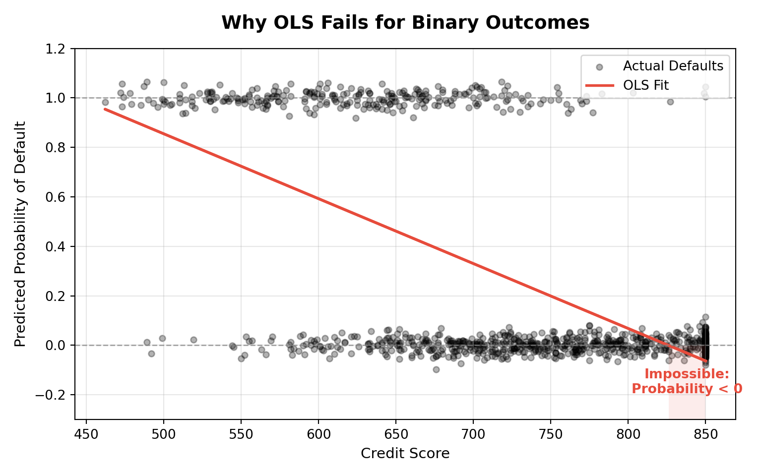

8.3 The Logit Function

In Section 8.2, we saw that modeling probability directly with a linear equation can produce impossible values (less than 0 or greater than 1) and ignores the way variance changes with the mean.

The fix is to apply a transformation that:

Expands the (0, 1) probability range to the entire real line,
Is reversible, so we can convert back to probabilities, and
Preserves the ordering of probabilities.

One transformation that checks all these boxes is the logit function.

8.3.1 Logit: A Link Between Probability and Linear Predictors

The logit function transforms the probability $\pi_i$ into a value on the entire real line: \[ \text{logit}(\pi_i) = \log\!\left(\frac{\pi_i}{1 - \pi_i}\right) = \beta_0 + \beta_1 X_i \]

This transformation:

Is monotonic (it preserves order),
Maps probabilities $\pi_i \in (0, 1)$ to $(-\infty, \infty)$, and
Solves the range issue of OLS by letting us fit a linear model in the transformed space.

By modeling the log-odds as a linear function of predictors and then inverting the transformation, we obtain valid predicted probabilities that remain within $[0,1]$.

Note

The logit function is defined as: \[ \text{logit}(\pi_i) = \log\!\left(\frac{\pi_i}{1 - \pi_i}\right) \] It models the log-odds of the outcome as a linear function of predictors.

8.3.2 From Log-Odds Back to Probability

While the model calculates linearly on the log-odds scale, we ultimately want to understand the probability of the outcome ($\pi_i$). To do this, we invert the logit function.

The inverse of the logit is the Sigmoid function (also called the logistic function):

\[ \pi_i = \frac{1}{1 + e^{-(\beta_0 + \beta_1 X_i)}} \]

This function takes our linear prediction ($\beta_0 + \beta_1 X_i$), which can range from $-\infty$ to $+\infty$, and “squashes” it into the range $(0, 1)$. This mathematical trick ensures that no matter how extreme our predictor values get, our predicted probability never exceeds 1 or drops below 0.

Figure 8.3: The Logistic Function showing the S-shape curve

8.3.3 Understanding the “S” Shape

The sigmoid function is not just a boundary enforcer; it fundamentally changes how we interpret the relationship between $X$ and $Y$. Unlike a straight line, the sigmoid curve is non-linear.

1. The Steep Middle (High Sensitivity) When the probability is near 0.5 (the “tipping point”), the curve is steepest. This means that small changes in the predictor $X$ result in large changes in the probability $\pi_i$.

Context: If a borrower is borderline (e.g., 50/50 chance of default), a small improvement in their credit score can drastically reduce their default risk.

2. The Flat Tails (Diminishing Returns) As the probability approaches 0 or 1, the curve flattens out (asymptotes). In these regions, even large changes in $X$ result in tiny changes in $\pi_i$.

Context: If a borrower has a near-perfect credit score (risk $\approx 0.01\%$), increasing their score further makes almost no difference to their probability of default. The model recognizes that they are already “maxed out” on safety.

This captures a realistic property of many binary outcomes: interventions are most effective when the outcome is uncertain.

This transformation lets us use a linear predictor on the log-odds scale and then recover valid probabilities.
This idea forms the basis of binary logistic regression, introduced next.

Visualizing the Difference

In OLS (Linear Regression), the slope is constant ($\beta_1$). In Logistic Regression, the “slope” (rate of change in probability) changes constantly—it is steepest at $\pi = 0.5$ and approaches zero at the extremes.

8.3.4 The Logistic Function and Its Shape (Code)

The following plot illustrates this behavior. Notice how the linear model (red dashed line) marches blindly past 0 and 1, while the logistic model (blue solid line) respects the boundaries and shows the characteristic “S” shape.

Figure 8.4: The Sigmoid ‘S-Curve’ vs. Linear Fit. The logistic model (blue solid line) respects the [0,1] probability bounds and captures the non-linear “diminishing returns” at the extremes, whereas the linear model (red dashed line) extends indefinitely.

R Code
Python Code

# Logistic vs Linear fit demo
set.seed(1)
# Grid of linear predictor values (η)
eta <- seq(-4, 4, length.out = 400)

# Logistic sigmoid: π(η)
pi  <- 1 / (1 + exp(-eta))

# Naive linear "probability" for comparison
# passes through (0, 0.5) with moderate slope
p_lin <- 0.5 + 0.25 * eta

df <- data.frame(
  eta    = eta,
  sigmoid = pi,
  linear  = p_lin
)

library(ggplot2)

ggplot(df, aes(x = eta)) +
  # Logistic S-curve
  geom_line(aes(y = sigmoid), linewidth = 1.4, color = "steelblue") +
  # Naive linear line
  geom_line(aes(y = linear), linewidth = 1.1, linetype = "dashed",
            color = "#E74C3C") +
  # Vertical marker for steepest change near π ≈ 0.5
  geom_segment(aes(x = 0, xend = 0,
                   y = plogis(-0.7), yend = plogis(0.7)),
               colour = "gray40", linewidth = 0.7) +
  annotate("text", x = 0.7, y = 0.55,
           label = "Steepest change\nat π ≈ 0.5",
           size = 3.5, hjust = 0, color = "gray30") +
  coord_cartesian(ylim = c(0, 1)) +
  scale_y_continuous(breaks = seq(0, 1, by = 0.25)) +
  labs(
    x = "Linear predictor (η = β0 + β1 X)",
    y = "Probability (π)",
    title = "The Sigmoid 'S-Curve' vs. Linear Fit",
    subtitle = "Logistic regression captures diminishing returns at the extremes",
    caption = "Blue: Logistic Sigmoid (Valid Probabilities). Red: Naive Linear (Violates Bounds)."
  ) +
  theme_minimal(base_size = 12) +
  theme(
    plot.title = element_text(hjust = 0.5, face = "bold", size = 14),
    plot.subtitle = element_text(hjust = 0.5, size = 11, colour = "gray40")
  )

import numpy as np
import matplotlib.pyplot as plt
from scipy.special import expit  # logistic / sigmoid

np.random.seed(1)

# Grid of linear predictor values (η)
eta = np.linspace(-4, 4, 400)

# Logistic sigmoid π(η)
pi = expit(eta)

# Naive linear "probability" (same as R: 0.5 + 0.25η)
p_lin = 0.5 + 0.25 * eta

plt.figure(figsize=(8, 5))

# Logistic S-curve
plt.plot(eta, pi, label="Logistic Sigmoid (Valid $\pi$)",
         linewidth=2.0, color="steelblue")

# Naive linear line
plt.plot(eta, p_lin, "--", label="Naive Linear (Violates Bounds)",
         linewidth=1.5, color="#E74C3C")

# Vertical marker around steepest change near π ≈ 0.5
y_lo, y_hi = expit(-0.7), expit(0.7)
plt.plot([0, 0], [y_lo, y_hi], color="gray40", linewidth=1.0)
plt.text(0.7, 0.55, "Steepest change\nat $\pi \\approx 0.5$",
         fontsize=10, color="gray30", ha="left", va="center")

plt.ylim(0, 1)
plt.yticks(np.arange(0, 1.01, 0.25))
plt.xlabel(r"Linear predictor ($\eta = \beta_0 + \beta_1 X$)")
plt.ylabel(r"Probability ($\pi$)")
plt.title("The Sigmoid 'S-Curve' vs. Linear Fit")
plt.grid(True, alpha=0.3)
plt.legend(loc="lower right")
plt.tight_layout()
plt.show()

8.4 Case Study: Understanding Financial Behaviors

Statistical models are most useful when they connect to a real-world problem. Here, we’ll use binary logistic regression to study financial behavior — specifically, the likelihood that a student defaults on a loan.

8.4.1 The Dataset

We’ll use the Logistic_Regression dataset (packaged in cookbook).

Predictors:
- credit_score (numeric, higher = lower risk)
- income (numeric, annual income in dollars)
- age (numeric)
- loan_amount (numeric, loan size)
- student (categorical: yes/no)
Outcome:
- defaulted (binary: 1 = default, 0 = no default)

Note

This is a binary classification problem: given a mix of continuous and categorical predictors, we want to predict whether a student defaults.

8.4.2 The Problem We’re Trying to Solve

Banks and lenders routinely face a critical decision:

Given a customer’s financial history, should we approve their loan application?

While this sounds like a simple “Yes” or “No” question, the reality is a complex game of probability and risk management.

1. The Balancing Act of Lending

Lending is a trade-off between two competing goals:

Maximizing Profit: The bank wants to lend to as many people as possible to earn interest.
Minimizing Loss: The bank wants to avoid lending to people who will not pay the money back (default).

If a bank is too strict, they reject good customers and lose profit. If they are too lenient, they lose their principal investment. The goal of Binary Logistic Regression here is not just to guess who defaults, but to quantify the risk ($\hat{\pi}_i$) so the bank can find the profitable “sweet spot.”

2. The Asymmetry of Errors

In this context, being wrong in one direction is much more expensive than being wrong in the other.

False Positive (Type I Error): The model predicts a customer will default, but they would have paid.
- Cost: The bank loses the potential interest (opportunity cost).
False Negative (Type II Error): The model predicts a customer is safe, but they default.
- Cost: The bank loses the entire loan amount.

Because a False Negative is usually much costlier than a False Positive, lenders need a model that outputs a precise probability (e.g., “There is an 18% chance this person defaults”). This allows them to set a custom decision threshold—perhaps they only approve loans if the risk of default is below 10%, rather than the standard 50%.

8.4.3 Study Design

Predictor types: both continuous (income, age, credit_score, loan_amount) and categorical (student status).
Outcome: binary (defaulted).
Sample size: dataset includes a few hundred observations (enough to illustrate the method).
Assumptions:
- Observations are independent.
- Predictors have a linear relationship with the log-odds of default.
- No perfect collinearity among predictors.

8.4.4 Applying Study Design to Our Case Study

Before we fit the model, we must prepare the data. In predictive modeling, this involves three critical steps: splitting, checking for imbalance, and handling outliers.

Why We Split the Data (Training vs. Testing)

A common mistake is to fit a model on all available data and then evaluate its performance on that same data. This leads to overfitting: the model memorizes the specific noise in the dataset rather than learning the underlying patterns.

To ensure our model generalizes to new, unseen borrowers, we split the data into two sets:

Training Set (e.g., 70%): Used to estimate the coefficients ($\hat{\beta}$). The model “sees” this data.
Testing Set (e.g., 30%): Used only to evaluate performance. The model never sees this data during fitting.

The Challenge of Class Imbalance

In loan default data, “success” (paying back the loan) is much more common than “failure” (defaulting). This is known as class imbalance.

If 95% of borrowers pay back their loans, a naive model could simply predict “No Default” for everyone and achieve 95% accuracy. However, this model is useless to the bank because it identifies zero risks.

To handle this during the split, we use stratified sampling. This ensures that the proportion of defaulters is exactly the same in both the training and testing sets, preventing the “rare” event from disappearing entirely in the test set.

Influential Points and Outliers

Logistic regression is sensitive to outliers (extreme values). A single borrower with an income of $10,000,000 or an age of 110 can pull the logistic curve disproportionately, biasing the results.

Before modeling, we should check for:

Data Entry Errors: (e.g., a credit score of 9000, which is impossible).
Extreme Leverage Points: Legitimate but extreme values that might need to be capped or investigated.

8.4.5 Data Preparation in Action

Below, we split the data while preserving the class balance (stratification) and encode the categorical variables.

R Code
Python Code

library(rsample) # Part of tidymodels for splitting
library(dplyr)

# 1. Check Class Imbalance
# Notice if defaults are rare (e.g., < 10%)
prop.table(table(BLR$defaulted))

# 2. Stratified Split
# We use 'strata = defaulted' to ensure both sets have the same % of defaults
set.seed(123)
split <- initial_split(BLR, prop = 0.70, strata = defaulted)

train_data <- training(split)
test_data  <- testing(split)

# 3. Verify the split
nrow(train_data)
nrow(test_data)

import pandas as pd
from sklearn.model_selection import train_test_split

# 1. Check Class Imbalance
print(df['defaulted'].value_counts(normalize=True))

# 2. Stratified Split
# We use 'stratify=y' to ensure both sets have the same % of defaults
X = df.drop(columns=['defaulted'])
y = df['defaulted']

X_train, X_test, y_train, y_test = train_test_split(
    X, y, 
    test_size=0.3, 
    random_state=123, 
    stratify=y  # Crucial for imbalanced data
)

# 3. Verify the split
print(f"Training set shape: {X_train.shape}")
print(f"Testing set shape: {X_test.shape}")

8.5 Fitting the Binary Logistic Regression Model

Now that we’ve prepared the data, we fit the model. Our goal is to estimate the unknown parameters ($\beta$) that link our predictors (like credit_score) to the probability of default.

8.5.1 Model Specification

We define the relationship between the predictors and the probability of default $\pi_i$ as:

\[ \log\!\left(\frac{\pi_i}{1 - \pi_i}\right) = \beta_0 + \beta_1\,\text{credit\_score}_i + \beta_2\,\text{income}_i + \dots + \beta_k X_{ki} \]

Here is what the parameters entail:

$\pi_i$: The probability that the $i$-th student defaults.
$\beta_0$ (The Intercept): The expected log-odds of default when all predictors are zero. (Often theoretical, as no one has 0 credit score).
$\beta_1, \dots, \beta_k$ (The Slopes): The change in the log-odds of default for a one-unit increase in the predictor, holding all other variables constant.

8.5.2 Fitting the Model

To estimate these $\beta$ parameters, we use Maximum Likelihood Estimation (MLE).

In R, we use the glm() function (Generalized Linear Model). Crucially, we must specify family = binomial.

Why family = binomial? Standard regression (OLS) assumes the target variable follows a Normal (Gaussian) distribution. However, our target is binary (0/1), which follows a Bernoulli/Binomial distribution. This argument tells the software to switch from “Least Squares” to “Maximum Likelihood” using the binomial distribution.
Why Logit? By default, family = binomial uses the logit link function. While other links exist (like probit), the logit is preferred for its interpretability (odds ratios) and mathematical properties.

R Code
Python Code

# Fit the model using Generalized Linear Model (glm)
# family = binomial automatically defaults to link = "logit"
fit_glm <- glm(defaulted ~ credit_score + income + age + loan_amount + student,
               data = BLR,
               family = binomial)

summary(fit_glm)

import statsmodels.api as sm

# 1. Define Predictors (X) and Target (y)
# Note: We access the R dataframe 'BLR' using 'r.BLR'
df = r.BLR
X = df[['credit_score', 'income', 'age', 'loan_amount', 'student']]
y = df['defaulted']

# 2. Add Intercept manually (Statsmodels does not add it by default)
X = sm.add_constant(X)

# 3. Fit the Logit model
model = sm.Logit(y, X).fit()

print(model.summary())

8.5.3 Model Output Interpretation

The output table provides the Estimate (the $\beta$ coefficients) for each predictor.

Positive Coefficient (+): As this variable increases, the log-odds of default increase (Higher Risk).
Negative Coefficient (-): As this variable increases, the log-odds of default decrease (Lower Risk).

In the next section, we will convert these raw log-odds into Odds Ratios, which are much easier to interpret for business decisions.

8.6 Interpreting Model Results: Log-Odds and Odds Ratios

In the previous section, we fit a model with several predictors. To clearly demonstrate how to interpret the coefficients, let’s focus on a simplified model using just two key variables: credit_score and income.

8.6.1 The “Log-Odds” Output

By default, logistic regression software outputs coefficients ($\hat{\beta}$) in log-odds.

R: The estimate column.
Python: The coef column.

While mathematically necessary, log-odds are difficult for humans to visualize. (e.g., “What does a -0.004 change in log-odds mean?”).

8.6.2 The “Odds Ratio” (OR)

To make these numbers interpretable, we exponentiate the coefficients: \[\text{OR} = e^{\hat{\beta}}\]

If $\text{OR} > 1$: The predictor is associated with higher odds of default.
If $\text{OR} < 1$: The predictor is associated with lower odds of default.
If $\text{OR} = 1$: No association.

Below, we fit the simplified model and calculate the Odds Ratios with 95% Confidence Intervals.

R Code
Python Code

# Fit a simplified model for clear interpretation
fit_simple <- glm(
  defaulted ~ credit_score + income,
  data = BLR,
  family = binomial(link = "logit")
)

# We use broom::tidy to easily extract coefficients and convert them
library(broom)
coef_table <- tidy(fit_simple, conf.int = TRUE, conf.level = 0.95)

# Calculate Odds Ratios (OR) by exponentiating estimates and CIs
coef_table$odds_ratio <- exp(coef_table$estimate)
coef_table$or_low     <- exp(coef_table$conf.low)
coef_table$or_high    <- exp(coef_table$conf.high)

# Display the table
knitr::kable(
  coef_table[, c("term","estimate","std.error","p.value","odds_ratio","or_low","or_high")],
  digits = 4,
  col.names = c("Term","Log-Odds (β)","SE","p","Odds Ratio","OR 2.5%","OR 97.5%")
)

import pandas as pd
import statsmodels.api as sm
import numpy as np

# Access the data from R
df = r.BLR
X = sm.add_constant(df[['credit_score', 'income']])
y = df['defaulted']

# Fit the simplified model
logit_model = sm.Logit(y, X).fit(disp=False)

# 1. Extract Parameters (Log-Odds)
params = logit_model.params
conf   = logit_model.conf_int()

# 2. Calculate Odds Ratios (OR)
# We exponentiate the log-odds to get the OR
odds_ratios = np.exp(params)
conf_or     = np.exp(conf)

# 3. Create a clean summary table
results_table = pd.DataFrame({
    "Log-Odds (β)": params,
    "p-value": logit_model.pvalues,
    "Odds Ratio": odds_ratios,
    "OR 2.5%": conf_or[0],
    "OR 97.5%": conf_or[1]
})

print(results_table.round(4))

Interpretation of the Output

Intercept: usually ignored in interpretation.
credit_score: If the coefficient is $\beta \approx -0.01$, then $\text{OR} \approx 0.99$.
- Meaning: For every 1-point increase in credit score, the odds of default are multiplied by 0.99 (a ~1% decrease), holding income constant.
income: If the $\text{OR} \approx 1.00$, the effect per dollar is tiny. In such cases, it is often useful to rescale the variable (e.g., income in $10k units) to see a meaningful effect size.

8.7 From Log-Odds to Probabilities (Simple Model)

To fully understand how the model converts abstract “log-odds” into a tangible “probability,” it is best to start with the simplest case: one predictor.

In a simple binary logistic regression, the relationship is:

\[ \hat{\pi} = \frac{1}{1 + e^{-(\hat{\beta}_0 + \hat{\beta}_1 X)}} \]

Below, we fit a model using only credit_score to predict default. We will then calculate the predicted probability ($\hat{\pi}$) for a student with a Low, Median, and High credit score.

R Code
Python Code

# 1. Fit a Simple Model (1 Predictor)
fit_simple <- glm(defaulted ~ credit_score, data = BLR, family = binomial)

# 2. Define Scenarios: Low, Median, and High Credit Score
# We pick the 25th, 50th, and 75th percentiles
qs <- quantile(BLR$credit_score, probs = c(0.25, 0.5, 0.75), na.rm = TRUE)

scenarios <- data.frame(
  scenario = c("Low (25th %)", "Median (50th %)", "High (75th %)"),
  credit_score = as.numeric(qs)
)

# 3. Calculate Linear Predictor (Log-Odds) and Probability
# type = "link" gives log-odds (eta)
# type = "response" gives probability (pi)
scenarios$log_odds <- predict(fit_simple, newdata = scenarios, type = "link")
scenarios$prob_pi  <- predict(fit_simple, newdata = scenarios, type = "response")

# Display Results
knitr::kable(
  scenarios,
  digits = 3,
  col.names = c("Scenario", "Credit Score", "Log-Odds (η)", "Probability (π)")
)

import pandas as pd
import statsmodels.api as sm
import numpy as np

# 1. Fit a Simple Model (1 Predictor)
# We define X with only credit_score
X_simple = sm.add_constant(df[['credit_score']])
y = df['defaulted']
model_simple = sm.Logit(y, X_simple).fit(disp=0)

# 2. Define Scenarios
qs = df['credit_score'].quantile([0.25, 0.5, 0.75]).values
scenarios = pd.DataFrame({
    'const': 1.0, 
    'credit_score': qs
}, index=["Low (25th %)", "Median (50th %)", "High (75th %)"])

# 3. Calculate Linear Predictor and Probability manually
# eta = beta0 + beta1 * score
eta = np.dot(scenarios, model_simple.params)
# pi = 1 / (1 + e^-eta)
pi  = 1 / (1 + np.exp(-eta))

# Display Results
results = pd.DataFrame({
    "Credit Score": scenarios['credit_score'],
    "Log-Odds (η)": eta,
    "Probability (π)": pi
})

print(results.round(3))

Interpretation

At Low Credit Score: The log-odds are likely positive (or less negative), resulting in a higher probability ($\pi$) of default.
At High Credit Score: The log-odds become strongly negative. Because of the exponent in the denominator ($e^{-\text{negative}}$ is large), the probability $\pi$ shrinks toward 0.

This demonstrates the inverse relationship: as credit score goes up, the probability of default goes down, following the S-curve shape we saw earlier.

Next Steps: Now that we understand the mechanics of the simple model, we can expand our view. Real-world problems are rarely caused by a single factor. In the following sections, we will add more variables (like income and student status) to build a multiple logistic regression model.

8.8 Data Preparation and Wrangling

Before we can train a model, we must bridge the gap between how data is collected and how a regression model consumes it. Raw data is often messy, incomplete, or stored in text formats that mathematical algorithms cannot process.

Data wrangling ensures our inputs are reliable (free of errors), complete (no missing values), and structured (numerical matrices). Without this step, even the most sophisticated algorithm will fail—a principle known as “Garbage In, Garbage Out.”

8.8.1 Handling Missing Data

Real-world datasets frequently have gaps—a borrower might leave the “Income” field blank. Logistic regression requires a complete set of observations; it cannot calculate a coefficient for a “blank” space.

We must first check the extent of the problem. If only a few rows have missing data, we typically remove them.

Strategies for Missing Values

When data is missing, you have three main options:

Deletion (Complete Case Analysis): If missingness is rare (<5% of data) and random, simply remove those rows. This is the most common approach in introductory texts.
Imputation: Replace missing values with the mean, median, or a value predicted by other variables. This preserves sample size but adds complexity.
Flagging: Create a new binary variable (e.g., income_missing = 1) to model the missingness explicitly.

8.8.2 Encoding Categorical Variables

Logistic regression works with matrices of numbers. It cannot mathematically multiply a coefficient $\beta$ by the text string “Married.”

To fix this, we perform One-Hot Encoding (or Dummy Encoding). This converts a categorical variable into a binary 0/1 flag.

Original: student = "Yes"
Encoded: student_yes = 1

Note on Multicollinearity: If a variable has two categories (Student: Yes/No), we only need one column (is_student). If we included both student_yes and student_no, they would be perfectly correlated, causing the math to break (the “Dummy Variable Trap”).

8.8.3 Splitting the Data

Finally, as discussed in the study design, we split our clean, encoded dataset into training and testing sets to evaluate performance fairly.

R Code
Python Code

library(dplyr)
library(rsample)

# 1. Handling Missing Data
# We check for NAs and, for this chapter, remove incomplete rows
sum(is.na(BLR)) 
BLR_clean <- na.omit(BLR)

# 2. Encoding
# R handles factor encoding automatically in glm(), 
# but it is good practice to ensure variables are factors.
BLR_clean <- BLR_clean %>%
  mutate(
    student = as.factor(student),
    married = as.factor(married),
    owns_home = as.factor(owns_home)
  )

# 3. Splitting (Stratified to handle class imbalance)
set.seed(123)
split <- initial_split(BLR_clean, prop = 0.7, strata = defaulted)
train_data <- training(split)
test_data  <- testing(split)

import pandas as pd
from sklearn.model_selection import train_test_split

# 1. Handling Missing Data
# Drop rows with any missing values
df_clean = df.dropna().copy()

# 2. Encoding Categorical Variables
# We use pd.get_dummies to convert text categories to 0s and 1s.
# drop_first=True prevents the "Dummy Variable Trap" (e.g., keeps 'student_Yes', drops 'student_No')
df_clean = pd.get_dummies(df_clean, columns=['student', 'married', 'owns_home'], drop_first=True)

# Display the new columns to verify
print(df_clean.head())

# 3. Splitting (Stratified)
X = df_clean.drop(columns=['defaulted'])
y = df_clean['defaulted']

X_train, X_test, y_train, y_test = train_test_split(
    X, y, test_size=0.3, random_state=123, stratify=y
)

8.9 Exploratory Data Analysis (EDA)

Before fitting a logistic regression, we need to understand the structure of our data. Exploratory analysis helps us spot patterns, distributions, and potential issues.

8.9.1 Classifying Variables

To select the appropriate modeling technique, we must first classify our variables. In this analysis, defaulted is our binary outcome, and the remaining variables serve as regressors (explanatory variables).

Variable	Type	Role	Description
`defaulted`	Categorical (Binary)	Outcome ($Y$)	$1=$ Default, $0=$ No Default
`credit_score`	Continuous (Integer)	Regressor ($X$)	Credit rating (300-850)
`income`	Continuous	Regressor ($X$)	Annual income in CAD
`age`	Continuous (Integer)	Regressor ($X$)	Borrower age in years
`loan_amount`	Continuous	Regressor ($X$)	Size of loan in CAD
`education_years`	Count / Discrete	Regressor ($X$)	Years of schooling
`married`	Categorical (Nominal)	Regressor ($X$)	Marital status
`owns_home`	Categorical (Nominal)	Regressor ($X$)	Home ownership status

8.9.2 Visualizing Distributions

Continuous regressors (e.g., credit_score, income) can be visualized with histograms or density plots, split by default status.
Categorical regressors (e.g., married, owns_home) can be compared with barplots of default rates.

8.9.3 Exploring Relationships with Binary Outcome

Boxplots or violin plots of credit_score by default status, or barplots of default rates by home ownership, help reveal potential relationships. We also check correlations among continuous regressors to watch for multicollinearity.

R Code
Python Code

library(ggplot2)
library(ggcorrplot)

# Boxplot of credit score by default
ggplot(BLR, aes(x = as.factor(defaulted), y = credit_score)) +
  geom_boxplot() +
  labs(x = "Defaulted", y = "Credit Score", 
       title = "Credit Score Distribution by Default Status")

# Barplot of default by home ownership
ggplot(BLR, aes(x = as.factor(owns_home), fill = as.factor(defaulted))) +
  geom_bar(position = "fill") +
  labs(x = "Owns Home", y = "Proportion", 
       fill = "Defaulted",
       title = "Default Rates by Home Ownership")

# Correlation heatmap (Numeric regressors only)
corr <- cor(BLR[,c("credit_score","income","education_years","age")])
ggcorrplot(corr, lab = TRUE)

import seaborn as sns
import matplotlib.pyplot as plt

# Boxplot credit score by default
sns.boxplot(data=df, x="defaulted", y="credit_score")
plt.title("Credit Score Distribution by Default Status")
plt.show()

# Barplot default by home ownership
sns.barplot(data=df, x="owns_home", y="defaulted", errorbar=None)
plt.title("Default Rates by Home Ownership")
plt.show()

# Correlation heatmap
corr = df[['credit_score','income','education_years','age']].corr()
sns.heatmap(corr, annot=True, cmap="coolwarm")
plt.title("Correlation Heatmap of Continuous Regressors")
plt.show()

8.10 Data Modelling

With EDA complete, we’re ready to formally specify our logistic regression model.

8.10.1 Choosing a Logistic Regression Model

The response variable is binary: defaulted $\in \{0,1\}$. Logistic regression is appropriate because it models the probability of the event occurring ($\pi_i$) rather than the raw outcome.

8.10.2 Defining the Probability Distribution

Unlike linear regression, we do not model $Y_i$ directly. Instead, we assume that the outcome follows a Bernoulli distribution:

\[ Y_i \sim \text{Bernoulli}(\pi_i) \] where $\pi_i$ is the probability that the $i$-th customer defaults.

8.10.3 Setting Up the Logistic Regression Equation

We link the regressors to the probability $\pi_i$ using the logit function:

\[\log\left(\frac{\pi_i}{1 - \pi_i}\right) = \beta_0 + \beta_1 X_{1i} + \beta_2 X_{2i} + \dots + \beta_k X_{ki} \]

8.10.4 The Missing Error Term ($\epsilon$)

You may notice a key difference here compared to OLS equations ($Y = \beta X + \epsilon$): there is no error term $\epsilon$ at the end of the equation.

In OLS, $\epsilon$ captures random noise around the mean.
In Logistic Regression, the randomness is inherent in the Bernoulli distribution of $Y$ itself. Once we know $\pi_i$ (the probability), the randomness comes from the “coin flip” of whether the event actually happens or not. We do not add an extra error term to the log-odds equation.

8.10.5 Counting the Parameters

If we fit a model using credit_score and income to predict default, we are estimating 3 parameters:

$\beta_0$: The intercept.
$\beta_1$: The coefficient for credit_score.
$\beta_2$: The coefficient for income.

Generally, if we have $k$ regressors, we estimate $k+1$ parameters.

R Code
Python Code

# Fit the full model
# We use family = binomial to indicate Y ~ Bernoulli(pi)
logit_model <- glm(defaulted ~ credit_score + income + married + owns_home,
                   data = BLR, family = binomial)
summary(logit_model)

import statsmodels.api as sm

# Define Regressors (X) and Outcome (y)
# Ensure categorical variables are encoded (if not done in wrangling step)
X = df[['credit_score','income','married_Yes','owns_home_Yes']] 
X = sm.add_constant(X)
y = df['defaulted']

logit_model = sm.Logit(y, X).fit()
print(logit_model.summary())

8.11 Estimation

Under a model with $k$ regressors, the coefficients $\beta_0,\beta_1,\ldots,\beta_k$ are unknown and must be estimated from the data.

8.11.1 Maximum Likelihood Estimation (MLE)

Because our outcome $Y_i$ follows a Bernoulli distribution with probability $\pi_i$, we cannot use Least Squares. Instead, we use Maximum Likelihood Estimation.

We seek the values of $\beta$ that maximize the likelihood of observing the data we actually collected. The likelihood function is:

\[ L(\boldsymbol\beta)=\prod_{i=1}^n \pi_i^{y_i}(1-\pi_i)^{1-y_i} \] Where $\pi_i$ is connected to our regressors via the inverse-logit:

\[\pi_i=\frac{e^{\beta_0 + \dots + \beta_k X_{ki}}}{1+e^{\beta_0 + \dots + \beta_k X_{ki}}} \] The computer solves this using an iterative algorithm (Newton-Raphson) to find the $\hat{\beta}$ values that make the observed defaults most probable.

8.12 Inference

After estimating a logistic regression model, we often want to know whether predictors are statistically significant — i.e., whether they have a meaningful relationship with the probability of default. In logistic regression, inference is based on the likelihood framework.

8.12.1 Wald Tests

The Wald test checks whether an individual coefficient is significantly different from zero. For example, we can test whether credit_score has a nonzero effect on the odds of default. The test statistic is the ratio of the estimated coefficient to its standard error. In our loan-default example, the model summary below reports Wald tests for both credit_score and income.

8.12.2 Likelihood Ratio Tests

We can also compare nested models (e.g., model with credit_score only vs. model with credit_score + income) using the likelihood ratio (LR) test. This evaluates whether adding predictors significantly improves model fit. The R and Python output below show an LR test comparing a model with only credit_score to a model with both credit_score and income.

8.12.3 Confidence Intervals

Finally, we often report confidence intervals for odds ratios. For example, if the odds ratio for credit score is 0.99 with a 95% CI [0.98, 0.995], we can say with confidence that higher credit scores reduce the odds of default.

R Code
Python Code

# Logistic regression
logit_model <- glm(defaulted ~ credit_score + income,
                   data = BLR, family = binomial)

# Wald test results are included in summary
summary(logit_model)

# Confidence intervals for odds ratios
exp(cbind(OR = coef(logit_model), confint(logit_model)))

# Likelihood ratio test for nested models
model1 <- glm(defaulted ~ credit_score, data = BLR, family = binomial)
anova(model1, logit_model, test = "Chisq")

import statsmodels.api as sm
import numpy as np
from scipy.stats import chi2

df = r.data['BLR'].copy()
df['defaulted'] = df['defaulted'].astype(int)

# Full model
X_full = sm.add_constant(df[['credit_score','income']])
y = df['defaulted']
model_full = sm.Logit(y, X_full).fit()

# Wald test (coeff / SE)
wald_stats = (model_full.params / model_full.bse)**2
print("Wald test chi2 values:\n", wald_stats)

# Confidence intervals for odds ratios
conf = model_full.conf_int()
odds_ratios = np.exp(model_full.params)
conf_exp = np.exp(conf)
print("Odds Ratios:\n", pd.DataFrame({"OR": odds_ratios,
                                      "2.5%": conf_exp[0],
                                      "97.5%": conf_exp[1]}))

# Likelihood ratio test vs simpler model
X_simple = sm.add_constant(df[['credit_score']])
model_simple = sm.Logit(y, X_simple).fit()

LR_stat = 2 * (model_full.llf - model_simple.llf)
df_diff = model_full.df_model - model_simple.df_model
p_value = chi2.sf(LR_stat, df_diff)
print(f"LR Test: chi2={LR_stat:.2f}, df={df_diff}, p={p_value:.4f}")

R Output
Python Output

library(lmtest)
library(broom)

# Fit the logistic regression model
logit_model <- glm(defaulted ~ credit_score + income,
                   data = BLR, family = binomial)

# ===================================
# 1. WALD TESTS (from model summary)
# ===================================
summary(logit_model)


Call:
glm(formula = defaulted ~ credit_score + income, family = binomial, 
    data = BLR)

Coefficients:
               Estimate Std. Error z value Pr(>|z|)    
(Intercept)   1.104e+01  8.348e-01  13.228  < 2e-16 ***
credit_score -1.492e-02  1.240e-03 -12.031  < 2e-16 ***
income       -2.907e-05  4.414e-06  -6.586 4.52e-11 ***
---
Signif. codes:  0 '***' 0.001 '**' 0.01 '*' 0.05 '.' 0.1 ' ' 1

(Dispersion parameter for binomial family taken to be 1)

    Null deviance: 1180.20  on 999  degrees of freedom
Residual deviance:  732.93  on 997  degrees of freedom
AIC: 738.93

Number of Fisher Scoring iterations: 6

# ===================================
# 2. ODDS RATIOS WITH CONFIDENCE INTERVALS
# ===================================
# Calculate odds ratios and confidence intervals
coef_table <- tidy(logit_model, conf.int = TRUE, conf.level = 0.95)
coef_table <- coef_table %>%
  mutate(
    odds_ratio = exp(estimate),
    or_lower = exp(conf.low),
    or_upper = exp(conf.high)
  )

# Display formatted table
knitr::kable(
  coef_table %>% 
    select(term, estimate, std.error, p.value, odds_ratio, or_lower, or_upper),
  digits = 4,
  col.names = c("Term", "Log-Odds (β)", "SE", "p-value", 
                "Odds Ratio", "OR 2.5%", "OR 97.5%"),
  caption = "Logistic Regression Coefficients with Odds Ratios"
)

Logistic Regression Coefficients with Odds Ratios
Term	Log-Odds (β)	SE	Odds Ratio	OR 2.5%	OR 97.5%
(Intercept)	11.0420	0.8348	62444.6652	12844.5451	340260.9478
credit_score	-0.0149	0.0012	0.9852	0.9827	0.9875
income	0.0000	0.0000	1.0000	1.0000	1.0000

# ===================================
# 3. LIKELIHOOD RATIO TEST
# ===================================
# Compare nested models
model_simple <- glm(defaulted ~ credit_score, data = BLR, family = binomial)
model_full <- glm(defaulted ~ credit_score + income, data = BLR, family = binomial)

# LR test
lr_test <- anova(model_simple, model_full, test = "Chisq")
print(lr_test)

Analysis of Deviance Table

Model 1: defaulted ~ credit_score
Model 2: defaulted ~ credit_score + income
  Resid. Df Resid. Dev Df Deviance  Pr(>Chi)    
1       998     787.73                          
2       997     732.93  1     54.8 1.334e-13 ***
---
Signif. codes:  0 '***' 0.001 '**' 0.01 '*' 0.05 '.' 0.1 ' ' 1

# Alternative: using lmtest package
lrtest(model_simple, model_full)

Likelihood ratio test

Model 1: defaulted ~ credit_score
Model 2: defaulted ~ credit_score + income
  #Df  LogLik Df Chisq Pr(>Chisq)    
1   2 -393.87                        
2   3 -366.47  1  54.8  1.334e-13 ***
---
Signif. codes:  0 '***' 0.001 '**' 0.01 '*' 0.05 '.' 0.1 ' ' 1

import pandas as pd
import statsmodels.api as sm
import numpy as np
from scipy.stats import chi2

# Prepare data
df = r.BLR.copy()
df['defaulted'] = df['defaulted'].astype(int)

# Fit the logistic regression model
X = sm.add_constant(df[['credit_score', 'income']])
y = df['defaulted']
logit_model = sm.Logit(y, X).fit()

Optimization terminated successfully.
         Current function value: 0.366466
         Iterations 7

# ===================================
# 1. MODEL SUMMARY (includes Wald tests)
# ===================================
print(logit_model.summary())

                           Logit Regression Results                           
==============================================================================
Dep. Variable:              defaulted   No. Observations:                 1000
Model:                          Logit   Df Residuals:                      997
Method:                           MLE   Df Model:                            2
Date:                Mon, 08 Dec 2025   Pseudo R-squ.:                  0.3790
Time:                        07:55:00   Log-Likelihood:                -366.47
converged:                       True   LL-Null:                       -590.10
Covariance Type:            nonrobust   LLR p-value:                 7.553e-98
================================================================================
                   coef    std err          z      P>|z|      [0.025      0.975]
--------------------------------------------------------------------------------
const           11.0420      0.835     13.228      0.000       9.406      12.678
credit_score    -0.0149      0.001    -12.031      0.000      -0.017      -0.012
income       -2.907e-05   4.41e-06     -6.586      0.000   -3.77e-05   -2.04e-05
================================================================================

# ===================================
# 2. ODDS RATIOS WITH CONFIDENCE INTERVALS
# ===================================
# Extract parameters and confidence intervals
params = logit_model.params
conf = logit_model.conf_int()
conf.columns = ['Lower', 'Upper']

# Calculate odds ratios
odds_ratios = pd.DataFrame({
    'Log-Odds (β)': params,
    'OR': np.exp(params),
    'OR Lower 95%': np.exp(conf['Lower']),
    'OR Upper 95%': np.exp(conf['Upper']),
    'p-value': logit_model.pvalues
})

print("\nOdds Ratios with 95% Confidence Intervals:")


Odds Ratios with 95% Confidence Intervals:

print(odds_ratios.round(4))

              Log-Odds (β)          OR  OR Lower 95%  OR Upper 95%  p-value
const              11.0420  62444.6652    12159.9124   320671.4057      0.0
credit_score       -0.0149      0.9852        0.9828        0.9876      0.0
income             -0.0000      1.0000        1.0000        1.0000      0.0

# ===================================
# 3. LIKELIHOOD RATIO TEST
# ===================================
# Fit simpler model for comparison
X_simple = sm.add_constant(df[['credit_score']])
model_simple = sm.Logit(y, X_simple).fit(disp=0)

# Calculate LR statistic
LR_stat = 2 * (logit_model.llf - model_simple.llf)
df_diff = logit_model.df_model - model_simple.df_model
p_value = chi2.sf(LR_stat, df_diff)

print("\n" + "="*50)


==================================================

print("Likelihood Ratio Test: Simple vs Full Model")

Likelihood Ratio Test: Simple vs Full Model

print("="*50)

==================================================

print(f"LR Statistic: {LR_stat:.4f}")

LR Statistic: 54.8003

print(f"Degrees of Freedom: {df_diff}")

Degrees of Freedom: 1.0

print(f"p-value: {p_value:.4f}")

p-value: 0.0000

print(f"Decision: {'Reject H0' if p_value < 0.05 else 'Fail to reject H0'}")

Decision: Reject H0

print(f"Interpretation: Income {'significantly' if p_value < 0.05 else 'does not'} improve model fit")

Interpretation: Income significantly improve model fit

8.12.4 Interpreting the Inference Results

The statistical tests above help us answer a fundamental question: Are our predictors truly associated with default risk, or could the observed patterns have occurred by chance?

Wald Tests: Individual Predictor Significance

The model summary shows that both credit score and income are highly significant (p < 0.001).

The coefficient for credit score is approximately −0.0149.
This means that for each 1-point increase in credit score, the log-odds of default decrease by about 0.015, holding income constant.
On the odds scale this corresponds to an odds ratio of about 0.985 per point, i.e., roughly a 1.5% reduction in the odds of default for each extra credit-score point.
The coefficient for income is about −2.9 × 10⁻⁵ per dollar.
On a more interpretable scale, a $10,000 increase in income changes the log-odds by about −0.29, giving an odds ratio of about 0.75.
In other words, each additional $10,000 of income reduces the odds of default by roughly 25%, holding credit score fixed.

The very small p-values for both predictors give strong evidence that these relationships are real, not artifacts of random variation.

Likelihood Ratio Test: Is the Full Model Better?

The likelihood ratio test compares our two-predictor model (credit score + income) against a simpler model with credit score alone. The test yields a chi-squared statistic of about 54.8 on 1 degree of freedom (p ≈ 1.3 × 10⁻¹³).

Interpretation: The tiny p-value indicates that adding income does significantly improve model fit beyond credit score alone. In other words, even after accounting for credit score, income still provides extra information about default risk.

Confidence Intervals for Odds Ratios

The 95% confidence interval for the credit score odds ratio is approximately [0.983, 0.988] per 1-point increase. Because this interval lies entirely below 1.0, we can be confident that higher credit scores have a genuine protective effect.

Scaling to a more meaningful change:

A 50-point increase in credit score multiplies the odds of default by about
0.47, with a 95% CI roughly [0.42, 0.53].
So we are 95% confident that increasing a borrower’s credit score by 50 points cuts their odds of default by about half.

For income, a $10,000 increase corresponds to an odds ratio of about 0.75, with a 95% CI roughly [0.69, 0.82]. Again, the interval lies entirely below 1.0, indicating a clear protective effect of higher income on default risk.

Practical Implications

These results suggest that both credit score and income play important roles in predicting default, with credit score exerting the larger effect. From a lender’s perspective:

Credit score provides a strong, easily interpretable signal: borrowers with higher scores are much less likely to default.
Income adds meaningful additional information: among borrowers with the same credit score, those with higher incomes still have substantially lower default risk.

In practice, a lender might prefer to include both variables in their risk model to balance predictive performance with interpretability.

8.13 Coefficient Interpretation

Once we’ve established that predictors matter, the next step is to interpret the coefficients in a meaningful way.

8.13.1 Odds Ratios and Their Meaning

Logistic regression coefficients are expressed in log-odds units. To make them interpretable, we exponentiate them to obtain odds ratios.

In our loan-default model, the estimated coefficient for credit score is about −0.0149, which corresponds to an odds ratio of roughly 0.985 per 1-point increase.
That means each extra point in credit score reduces the odds of default by about 1.5%.

Scaling makes interpretation clearer:

A 50-point increase in credit score multiplies the odds of default by about 0.47, i.e., it roughly cuts the odds of default in half.
For income, the coefficient per dollar is very small, but over a $10,000 increase it corresponds to an odds ratio of about 0.75.
So each extra $10,000 of income lowers the odds of default by about 25%.

8.13.2 Pitfalls in Interpretation

It’s important to remember that odds ratios are multiplicative, not additive. This means the effect on probability depends on the baseline. For example:

Going from a 40% chance of default to 30% is a big shift,
But the same odds ratio may translate into a much smaller change if the baseline probability is already low (e.g., from 5% to 4%).

Clear communication requires translating odds ratios back into probability changes for meaningful scenarios.

8.13.3 Example from Loan Default Dataset

In our fitted model (see the odds-ratio table), we estimate that:

A 50-point increase in credit score multiplies the odds of default by about 0.47
(roughly a 53% reduction in the odds of default).
A $10,000 increase in income multiplies the odds of default by about 0.75
(about a 25% reduction in the odds), holding credit score constant.

We can present this in plain English:

“Compared to an otherwise similar borrower with a credit score 50 points lower, a higher-score borrower has about half the odds of default.
Likewise, borrowers who earn $10,000 more per year have roughly 25% lower odds of default, even after accounting for credit score.”

R Code
Python Code

# Logistic regression 
logit_model <- glm(defaulted ~ credit_score + income, data = BLR, family = binomial) 

# Odds ratios and CI 
odds_ratios <- exp(cbind(OR = coef(logit_model), confint(logit_model))) odds_ratios 

# Example: probability at credit_score = 600 vs 700 
new_data <- data.frame(credit_score = c(600, 700), income = mean(BLR$income)) predict(logit_model, newdata = new_data, type = "response")

# Odds ratios
params = model_full.params
conf = model_full.conf_int()
odds_ratios = np.exp(params)
conf_exp = np.exp(conf)
print(pd.DataFrame({"OR": odds_ratios,
                    "2.5%": conf_exp[0],
                    "97.5%": conf_exp[1]}))

# Example: probability at 600 vs 700 credit score
test_data = pd.DataFrame({
    "const": 1,
    "credit_score": [600, 700],
    "income": [df['income'].mean(), df['income'].mean()]
})
print(model_full.predict(test_data))

8.13.4 Visualizing Predicted Probabilities

To make these odds ratios more concrete, we can plot predicted probabilities across the range of credit scores. This shows the characteristic S-shaped curve of logistic regression.

R Code
Python Code

# Fit simple model with credit score only for clear visualization
model_simple <- glm(defaulted ~ credit_score, data = BLR, family = binomial)

# Create sequence of credit scores for prediction
credit_seq <- seq(min(BLR$credit_score), max(BLR$credit_score), length.out = 200)
pred_df <- data.frame(credit_score = credit_seq)

# Get predicted probabilities with confidence intervals
pred_df$prob <- predict(model_simple, newdata = pred_df, type = "response")

# Calculate confidence intervals on the linear predictor scale, then transform
pred_link <- predict(model_simple, newdata = pred_df, type = "link", se.fit = TRUE)
pred_df$lower <- plogis(pred_link$fit - 1.96 * pred_link$se.fit)
pred_df$upper <- plogis(pred_link$fit + 1.96 * pred_link$se.fit)

# Add reference lines for key credit scores
ref_scores <- c(400, 500, 600, 700, 800)
ref_probs <- predict(model_simple, 
                     newdata = data.frame(credit_score = ref_scores),
                     type = "response")

# Create the plot
ggplot(pred_df, aes(x = credit_score, y = prob)) +
  # Confidence interval ribbon
  geom_ribbon(aes(ymin = lower, ymax = upper), fill = "#3498db", alpha = 0.2) +
  # Predicted probability curve
  geom_line(color = "#2C3E50", linewidth = 1.5) +
  # Actual data points (jittered for visibility)
  geom_jitter(data = BLR, 
              aes(x = credit_score, y = as.numeric(as.character(defaulted))),
              height = 0.02, alpha = 0.2, size = 0.8, color = "gray30") +
  # Reference lines for key credit scores
  geom_segment(data = data.frame(x = ref_scores, y = ref_probs),
               aes(x = x, xend = x, y = 0, yend = y),
               linetype = "dotted", color = "#E74C3C", alpha = 0.6) +
  geom_point(data = data.frame(x = ref_scores, y = ref_probs),
             aes(x = x, y = y), color = "#E74C3C", size = 3) +
  # Annotations for key points
  annotate("text", x = 400, y = ref_probs[1] + 0.08, 
           label = sprintf("Score 400\nP(default) = %.1f%%", ref_probs[1]*100),
           size = 3, color = "#E74C3C", fontface = "bold") +
  annotate("text", x = 700, y = ref_probs[4] - 0.08, 
           label = sprintf("Score 700\nP(default) = %.1f%%", ref_probs[4]*100),
           size = 3, color = "#E74C3C", fontface = "bold") +
  # Labels and theme
  labs(
    title = "The S-Curve: How Credit Score Affects Default Probability",
    subtitle = "Shaded area shows 95% confidence interval",
    x = "Credit Score",
    y = "Predicted Probability of Default"
  ) +
  scale_y_continuous(labels = scales::percent_format(), limits = c(0, 1)) +
  theme_minimal(base_size = 12) +
  theme(
    plot.title = element_text(hjust = 0.5, face = "bold", size = 14),
    plot.subtitle = element_text(hjust = 0.5, size = 10, color = "gray40")
  )

Warning: Removed 492 rows containing missing values or values outside the scale range
(`geom_point()`).

Warning: Removed 1 row containing missing values or values outside the scale range
(`geom_text()`).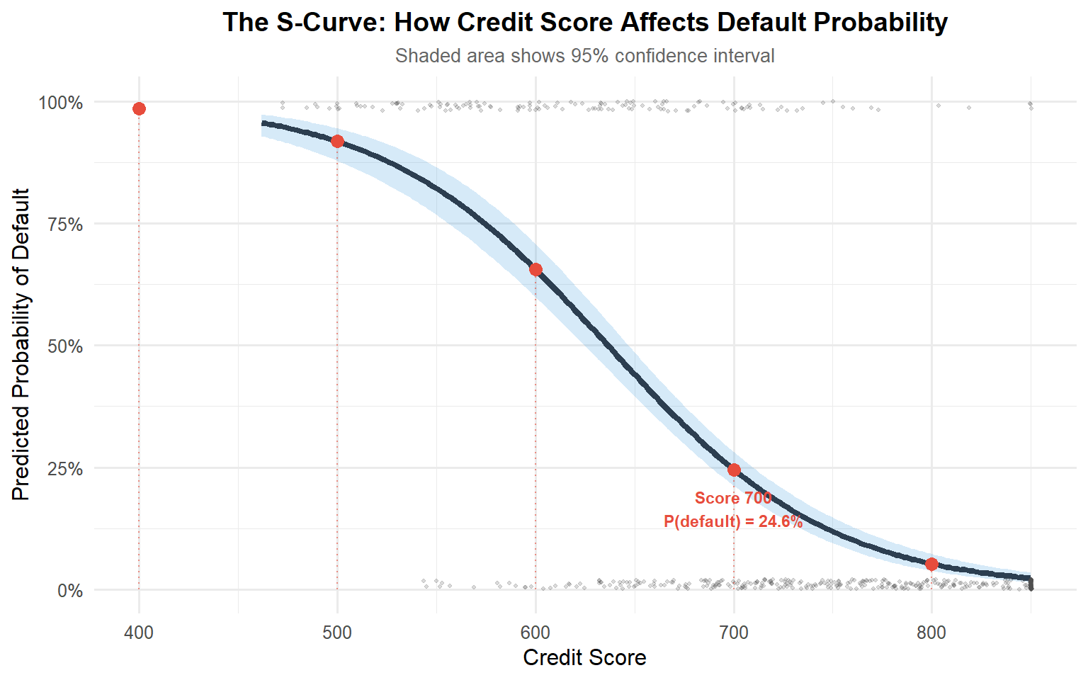

Figure 8.5: Predicted Probability of Default by Credit Score

#| label: fig-prob-curve-credit-py
#| fig-cap: "Predicted Probability of Default by Credit Score (Python)"
#| fig-width: 8
#| fig-height: 5

import pandas as pd
import numpy as np
import matplotlib.pyplot as plt
import statsmodels.api as sm
from scipy.special import expit

# Prepare data
df = r.BLR.copy()
df['defaulted'] = df['defaulted'].astype(int)

# Fit simple model with credit score only
X_simple = sm.add_constant(df[['credit_score']])
y = df['defaulted']
model_simple = sm.Logit(y, X_simple).fit(disp=0)

# Create sequence for prediction
credit_seq = np.linspace(df['credit_score'].min(), df['credit_score'].max(), 200)
pred_df = pd.DataFrame({'const': 1, 'credit_score': credit_seq})

# Get predictions (probabilities directly)
pred_probs = model_simple.predict(pred_df)

# Calculate confidence intervals manually
# Get linear predictor (log-odds) and its standard error
pred_logit = model_simple.predict(pred_df, linear=True)

C:\Users\aviv\AppData\Local\R\cache\R\RETICU~1\uv\cache\ARCHIV~1\9JLF1J~1\Lib\site-packages\statsmodels\discrete\discrete_model.py:530: FutureWarning: linear keyword is deprecated, use which="linear"
  warnings.warn(msg, FutureWarning)

# Get variance-covariance matrix and calculate SE
X_pred = pred_df.values
vcov = model_simple.cov_params()
se_logit = np.sqrt(np.diag(X_pred @ vcov @ X_pred.T))

# Transform to probability scale using inverse logit
lower_ci = expit(pred_logit - 1.96 * se_logit)
upper_ci = expit(pred_logit + 1.96 * se_logit)

# Create the plot
fig, ax = plt.subplots(figsize=(8, 5))

# Confidence interval
ax.fill_between(credit_seq, lower_ci, upper_ci,
                alpha=0.2, color='#3498db', label='95% CI')

# Predicted probability curve
ax.plot(credit_seq, pred_probs, color='#2C3E50', linewidth=2.5, 
        label='Predicted Probability')

# Actual data points (jittered)
np.random.seed(42)
jitter = np.random.normal(0, 0.02, size=len(df))
ax.scatter(df['credit_score'], df['defaulted'] + jitter, 
           alpha=0.2, s=10, color='gray', label='Actual Data')

# Reference points for key credit scores
ref_scores = np.array([400, 500, 600, 700, 800])
ref_df = pd.DataFrame({'const': 1, 'credit_score': ref_scores})
ref_probs = model_simple.predict(ref_df)

# Add reference lines
for score, prob in zip(ref_scores, ref_probs):
    ax.plot([score, score], [0, prob], ':', color='#E74C3C', alpha=0.6, linewidth=1)
    ax.plot(score, prob, 'o', color='#E74C3C', markersize=8)

# Annotations for extreme points
ax.text(400, ref_probs[0] + 0.08, 
        f'Score 400\nP(default) = {ref_probs[0]*100:.1f}%',
        ha='center', fontsize=9, color='#E74C3C', fontweight='bold')
ax.text(700, ref_probs[3] - 0.08, 
        f'Score 700\nP(default) = {ref_probs[3]*100:.1f}%',
        ha='center', fontsize=9, color='#E74C3C', fontweight='bold')

# Labels and styling
ax.set_xlabel('Credit Score', fontsize=11)
ax.set_ylabel('Predicted Probability of Default', fontsize=11)
ax.set_title('The S-Curve: How Credit Score Affects Default Probability', 
             fontsize=14, fontweight='bold', pad=15)
ax.text(0.5, 1.02, 'Shaded area shows 95% confidence interval',
        transform=ax.transAxes, ha='center', fontsize=9, color='gray')
ax.set_ylim(0, 1)

(0.0, 1.0)

ax.yaxis.set_major_formatter(plt.FuncFormatter(lambda y, _: f'{y:.0%}'))
ax.legend(loc='upper right', framealpha=0.9)
ax.grid(True, alpha=0.3)
plt.tight_layout()
plt.show()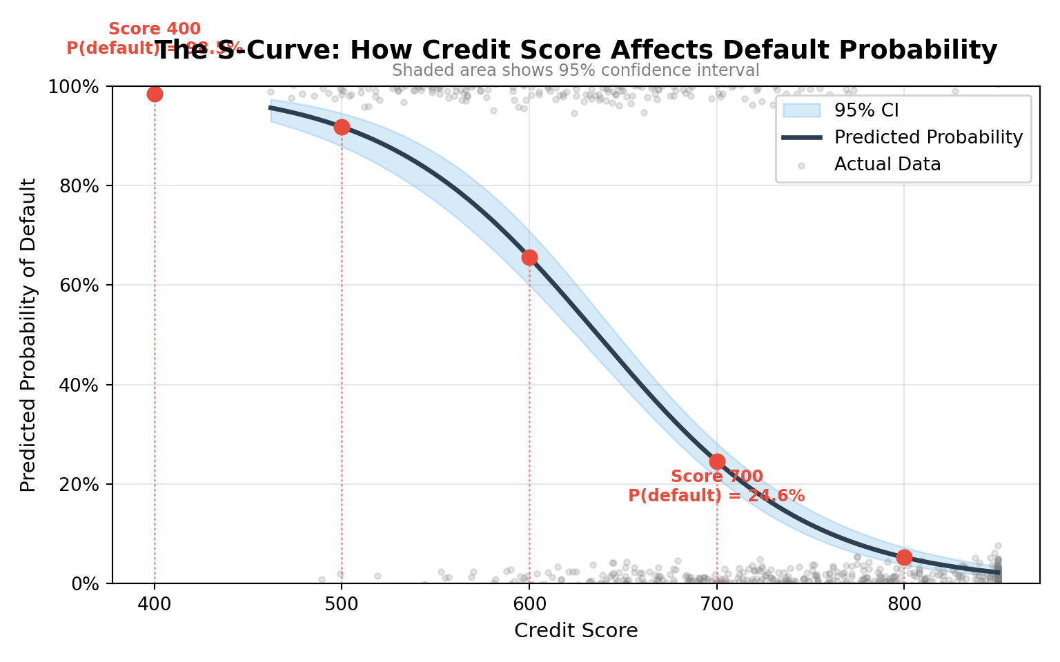

Interpretation: The plot reveals the nonlinear relationship between credit score and default probability. In our fitted model, a borrower with a credit score of 400 has an estimated default probability of about 98%, whereas a borrower with a score of 700 has a default probability of only about 25%.

Notice how the curve is steepest in the middle of the credit-score range: in that region, relatively small improvements in credit score translate into large reductions in default risk. At the extremes (very low or very high scores), additional changes in credit score have diminishing marginal effects on the predicted probability.

8.14 Predictions

Once we’ve fit a logistic regression model, we can use it to generate predicted probabilities of default for each customer. These probabilities fall between 0 and 1 and tell us how likely the model thinks it is that a customer will default given their predictors.

8.14.1 Predicted Probabilities vs. Predicted Classes

Predicted probabilities can be turned into class predictions (default vs. no default) by applying a threshold, usually 0.5. Customers with probability ≥ 0.5 are classified as “default,” and those below as “no default.”

But in practice, the choice of threshold matters. If we lower the threshold to 0.3, we’ll catch more actual defaulters (higher sensitivity) but at the cost of more false alarms (lower specificity).

8.14.2 Evaluating Performance

To judge prediction quality, we use metrics such as:

Accuracy: proportion of correct predictions.
Sensitivity (recall): proportion of true defaults correctly identified.
Specificity: proportion of true non-defaults correctly identified.
ROC curve & AUC: performance across all thresholds, not just one.

For our loan dataset, we might find that the model predicts non-defaults very well (high specificity) but misses some defaults (lower sensitivity). This trade-off is a central theme in logistic regression applications.

In the code below, we compute a confusion matrix at a 0.5 threshold and plot the ROC curve with its AUC for our loan default model.

R Code
Python Code

# Logistic regression model
logit_model <- glm(defaulted ~ credit_score + income,
                   data = BLR, family = binomial)

library(dplyr)
library(yardstick)
library(ggplot2)

# Add predicted probabilities and classes to BLR
BLR <- BLR %>%
  mutate(
    pred_prob  = predict(logit_model, type = "response"),
    pred_class = if_else(pred_prob >= 0.5, 1, 0)
  )

# Build results tibble for yardstick
results <- BLR %>%
  transmute(
    truth     = factor(defaulted, levels = c(0, 1)),
    predicted = factor(pred_class, levels = c(0, 1)),
    pred_prob = pred_prob
  )

# -----------------------------
# 1. CONFUSION MATRIX & METRICS
# -----------------------------
cm <- conf_mat(results, truth, predicted)
cm          # 2x2 confusion matrix

# Accuracy, sensitivity, specificity, precision, F1
metrics <- metric_set(accuracy, sens, spec, precision, f_meas)
metrics(results, truth, predicted)

# -----------------------------
# 2. ROC CURVE & AUC
# -----------------------------
roc_df  <- roc_curve(results, truth, pred_prob)
roc_auc <- roc_auc(results, truth, pred_prob)
roc_auc  # prints the AUC value

autoplot(roc_df) +
  labs(
    title = "ROC Curve for Loan Default Model",
    subtitle = "Area under the curve (AUC) summarizes performance across thresholds"
  )

from sklearn.metrics import confusion_matrix, classification_report, roc_curve, auc
import matplotlib.pyplot as plt
import statsmodels.api as sm

df = r.data['BLR'].copy()
df['defaulted'] = df['defaulted'].astype(int)

X = sm.add_constant(df[['credit_score','income']])
y = df['defaulted']
logit_model = sm.Logit(y, X).fit()
df['pred_prob'] = logit_model.predict(X)
df['pred_class'] = (df['pred_prob'] > 0.5).astype(int)

# Confusion matrix & metrics
print(confusion_matrix(y, df['pred_class']))
print(classification_report(y, df['pred_class']))

# ROC curve
fpr, tpr, thresholds = roc_curve(y, df['pred_prob'])
roc_auc = auc(fpr, tpr)

plt.plot(fpr, tpr, label=f"AUC = {roc_auc:.2f}")
plt.plot([0,1], [0,1], linestyle="--", color="grey")
plt.xlabel("False Positive Rate")
plt.ylabel("True Positive Rate")
plt.title("ROC Curve for Loan Default Model")
plt.legend()
plt.show()

R Output
Python Output

          Truth
Prediction   0   1
         0 657 106
         1  66 171

# A tibble: 5 × 3
  .metric   .estimator .estimate
  <chr>     <chr>          <dbl>
1 accuracy  binary         0.828
2 sens      binary         0.909
3 spec      binary         0.617
4 precision binary         0.861
5 f_meas    binary         0.884

# A tibble: 1 × 3
  .metric .estimator .estimate
  <chr>   <chr>          <dbl>
1 roc_auc binary         0.109

Confusion matrix (threshold 0.5):

[[657  66]
 [106 171]]


Classification report:

              precision    recall  f1-score   support

           0       0.86      0.91      0.88       723
           1       0.72      0.62      0.67       277

    accuracy                           0.83      1000
   macro avg       0.79      0.76      0.77      1000
weighted avg       0.82      0.83      0.82      1000


AUC: 0.891

8.15 Goodness of Fit & Model Selection

Evaluating whether our model is a “good” fit is just as important as making predictions. For logistic regression, the diagnostics differ from OLS.

8.15.1 Pseudo R-Squared Measures

Because we don’t have the same notion of variance explained as in OLS, we use pseudo R² measures (e.g., McFadden’s R²). These are useful for comparison, but don’t carry the same interpretation as R² in linear regression.

8.15.2 Analysis of Deviance

We can compare models using the deviance statistic, which measures how well the model fits relative to a saturated model. Lower deviance indicates better fit. Nested models (e.g., one with credit_score only vs. one with credit_score + income) can be compared using a likelihood ratio test.

8.15.3 Information Criteria

Another approach is to use information criteria such as:

AIC (Akaike Information Criterion)
BIC (Bayesian Information Criterion)

Both balance fit and complexity: lower AIC or BIC means a better trade-off. AIC tends to favor more complex models; BIC penalizes complexity more heavily.

For the loan default dataset, the diagnostics tell a clear story. The model with credit score + income (Model 2) fits substantially better than the credit-score-only model (Model 1): the likelihood ratio test is highly significant, and both AIC and BIC are lower for Model 2.

Adding education_years (Model 3) yields only a very small additional improvement in fit. AIC changes little and BIC actually prefers the simpler two-predictor model, since it penalizes extra parameters more heavily. In practice, we would typically choose Model 2 as a good balance between predictive performance and parsimony.

R Code
Python Code

# Fit models
model1 <- glm(defaulted ~ credit_score, data = BLR, family = binomial)
model2 <- glm(defaulted ~ credit_score + income, data = BLR, family = binomial)

# Compare deviance (likelihood ratio test)
anova(model1, model2, test = "Chisq")

# Pseudo R-squared
library(pscl)
pR2(model2)

# AIC and BIC
AIC(model1, model2)
BIC(model1, model2)

import statsmodels.api as sm

df = r.data['BLR'].copy()
df['defaulted'] = df['defaulted'].astype(int)

# Model 1: credit score only
X1 = sm.add_constant(df[['credit_score']])
model1 = sm.Logit(df['defaulted'], X1).fit()

# Model 2: credit score + income
X2 = sm.add_constant(df[['credit_score','income']])
model2 = sm.Logit(df['defaulted'], X2).fit()

# Likelihood ratio test
LR_stat = 2 * (model2.llf - model1.llf)
df_diff = model2.df_model - model1.df_model
from scipy.stats import chi2
p_value = chi2.sf(LR_stat, df_diff)

print("Likelihood Ratio Test:", LR_stat, "df:", df_diff, "p:", p_value)

# AIC & BIC
print("Model 1 AIC/BIC:", model1.aic, model1.bic)
print("Model 2 AIC/BIC:", model2.aic, model2.bic)

R Code
Python Code

library(pscl)  # For pseudo R-squared

Classes and Methods for R originally developed in the
Political Science Computational Laboratory
Department of Political Science
Stanford University (2002-2015),
by and under the direction of Simon Jackman.
hurdle and zeroinfl functions by Achim Zeileis.

library(broom)

# Fit models for comparison
model1 <- glm(defaulted ~ credit_score, data = BLR, family = binomial)
model2 <- glm(defaulted ~ credit_score + income, data = BLR, family = binomial)
model3 <- glm(defaulted ~ credit_score + income + education_years, 
              data = BLR, family = binomial)

# ===================================
# 1. PSEUDO R-SQUARED MEASURES
# ===================================
cat("\n=== Pseudo R-Squared Measures ===\n")


=== Pseudo R-Squared Measures ===

pr2_model2 <- pR2(model2)

fitting null model for pseudo-r2

print(pr2_model2)

         llh      llhNull           G2     McFadden         r2ML         r2CU 
-366.4661306 -590.0975621  447.2628631    0.3789737    0.3606242    0.5205456

# ===================================
# 2. DEVIANCE COMPARISON (Analysis of Deviance)
# ===================================
cat("\n=== Analysis of Deviance ===\n")


=== Analysis of Deviance ===

anova(model1, model2, model3, test = "Chisq")

Analysis of Deviance Table

Model 1: defaulted ~ credit_score
Model 2: defaulted ~ credit_score + income
Model 3: defaulted ~ credit_score + income + education_years
  Resid. Df Resid. Dev Df Deviance  Pr(>Chi)    
1       998     787.73                          
2       997     732.93  1    54.80 1.334e-13 ***
3       996     730.30  1     2.63    0.1049    
---
Signif. codes:  0 '***' 0.001 '**' 0.01 '*' 0.05 '.' 0.1 ' ' 1

# ===================================
# 3. INFORMATION CRITERIA (AIC & BIC)
# ===================================
cat("\n=== Model Comparison: AIC and BIC ===\n")


=== Model Comparison: AIC and BIC ===

# Create comparison table
model_comparison <- data.frame(
  Model = c("Model 1: credit_score only",
            "Model 2: + income",
            "Model 3: + education_years"),
  AIC = c(AIC(model1), AIC(model2), AIC(model3)),
  BIC = c(BIC(model1), BIC(model2), BIC(model3)),
  Deviance = c(deviance(model1), deviance(model2), deviance(model3)),
  Df = c(model1$df.residual, model2$df.residual, model3$df.residual)
)

knitr::kable(model_comparison, digits = 2,
             caption = "Model Comparison: AIC, BIC, and Deviance")

Model Comparison: AIC, BIC, and Deviance
Model	AIC	BIC	Deviance	Df
Model 1: credit_score only	791.73	801.55	787.73	998
Model 2: + income	738.93	753.66	732.93	997
Model 3: + education_years	738.30	757.93	730.30	996

# Find best model by each criterion
cat("\nBest model by AIC:", model_comparison$Model[which.min(model_comparison$AIC)])


Best model by AIC: Model 3: + education_years

cat("\nBest model by BIC:", model_comparison$Model[which.min(model_comparison$BIC)])


Best model by BIC: Model 2: + income

# ===================================
# 4. VISUALIZATION
# ===================================
library(ggplot2)

# Reshape for plotting
comparison_long <- model_comparison %>%
  tidyr::pivot_longer(cols = c(AIC, BIC), 
                      names_to = "Criterion", 
                      values_to = "Value")

ggplot(comparison_long, aes(x = Model, y = Value, fill = Criterion)) +
  geom_bar(stat = "identity", position = "dodge") +
  scale_fill_manual(values = c("AIC" = "#3498db", "BIC" = "#e74c3c")) +
  labs(title = "Model Comparison: AIC vs BIC",
       subtitle = "Lower values indicate better model fit",
       x = NULL, y = "Information Criterion Value") +
  theme_minimal() +
  theme(axis.text.x = element_text(angle = 15, hjust = 1),
        plot.title = element_text(hjust = 0.5, face = "bold"))

import pandas as pd
import statsmodels.api as sm
import numpy as np
import matplotlib.pyplot as plt
from scipy.stats import chi2


# Prepare data
df = r.BLR.copy()
df['defaulted'] = df['defaulted'].astype(int)

# Fit three models for comparison
# Model 1: credit_score only
X1 = sm.add_constant(df[['credit_score']])
model1 = sm.Logit(df['defaulted'], X1).fit(disp=0)

# Model 2: credit_score + income
X2 = sm.add_constant(df[['credit_score', 'income']])
model2 = sm.Logit(df['defaulted'], X2).fit(disp=0)

# Model 3: credit_score + income + education_years
X3 = sm.add_constant(df[['credit_score', 'income', 'education_years']])
model3 = sm.Logit(df['defaulted'], X3).fit(disp=0)

# ===================================
# 1. PSEUDO R-SQUARED MEASURES
# ===================================
print("\n" + "="*50)


==================================================

print("Pseudo R-Squared Measures (Model 2)")

Pseudo R-Squared Measures (Model 2)

print("="*50)

==================================================

print(f"McFadden's R²: {model2.prsquared:.4f}")

McFadden's R²: 0.3790

print(f"Log-Likelihood: {model2.llf:.2f}")

Log-Likelihood: -366.47

print(f"Null Log-Likelihood: {model2.llnull:.2f}")

Null Log-Likelihood: -590.10

# ===================================
# 2. LIKELIHOOD RATIO TESTS
# ===================================
print("\n" + "="*50)


==================================================

print("Likelihood Ratio Tests")

Likelihood Ratio Tests

print("="*50)

==================================================

# Model 1 vs Model 2
lr_12 = 2 * (model2.llf - model1.llf)
df_12 = model2.df_model - model1.df_model
p_12 = chi2.sf(lr_12, df_12)

print(f"\nModel 1 vs Model 2:")


Model 1 vs Model 2:

print(f"  LR Statistic: {lr_12:.4f}, df: {df_12}, p-value: {p_12:.4f}")

  LR Statistic: 54.8003, df: 1.0, p-value: 0.0000

# Model 2 vs Model 3
lr_23 = 2 * (model3.llf - model2.llf)
df_23 = model3.df_model - model2.df_model
p_23 = chi2.sf(lr_23, df_23)

print(f"\nModel 2 vs Model 3:")


Model 2 vs Model 3:

print(f"  LR Statistic: {lr_23:.4f}, df: {df_23}, p-value: {p_23:.4f}")

  LR Statistic: 2.6295, df: 1.0, p-value: 0.1049

# ===================================
# 3. INFORMATION CRITERIA (AIC & BIC)
# ===================================
print("\n" + "="*50)


==================================================

print("Model Comparison: AIC and BIC")

Model Comparison: AIC and BIC

print("="*50)

==================================================

comparison = pd.DataFrame({
    'Model': ['Model 1: credit_score only',
              'Model 2: + income',
              'Model 3: + education_years'],
    'AIC': [model1.aic, model2.aic, model3.aic],
    'BIC': [model1.bic, model2.bic, model3.bic],
    'Pseudo R²': [model1.prsquared, model2.prsquared, model3.prsquared]
})

print(comparison.round(2))

                        Model     AIC     BIC  Pseudo R²
0  Model 1: credit_score only  791.73  801.55       0.33
1           Model 2: + income  738.93  753.66       0.38
2  Model 3: + education_years  738.30  757.93       0.38

print(f"\nBest model by AIC: {comparison.loc[comparison['AIC'].idxmin(), 'Model']}")


Best model by AIC: Model 3: + education_years

print(f"Best model by BIC: {comparison.loc[comparison['BIC'].idxmin(), 'Model']}")

Best model by BIC: Model 2: + income

# ===================================
# 4. VISUALIZATION
# ===================================
fig, (ax1, ax2) = plt.subplots(1, 2, figsize=(12, 5))

# AIC comparison
ax1.bar(range(3), comparison['AIC'], color='#3498db', alpha=0.7)
ax1.set_xticks(range(3))
ax1.set_xticklabels(['Model 1', 'Model 2', 'Model 3'])
ax1.set_ylabel('AIC')
ax1.set_title('AIC Comparison\n(Lower is Better)', fontweight='bold')
ax1.grid(axis='y', alpha=0.3)

# BIC comparison
ax2.bar(range(3), comparison['BIC'], color='#e74c3c', alpha=0.7)
ax2.set_xticks(range(3))
ax2.set_xticklabels(['Model 1', 'Model 2', 'Model 3'])
ax2.set_ylabel('BIC')
ax2.set_title('BIC Comparison\n(Lower is Better)', fontweight='bold')
ax2.grid(axis='y', alpha=0.3)

plt.tight_layout()
plt.show()

8.16 Model Diagnostics

Once we’ve estimated our logistic regression model, it’s important to check whether the model is well-specified and whether there are any problematic observations influencing the results. Diagnostics help us assess whether our predictions are trustworthy and whether model assumptions are being violated.

8.16.1 Deviance Residuals

In logistic regression, we don’t have “raw residuals” like in OLS. Instead, we use deviance residuals, which measure how far off each predicted probability is from the actual outcome. Large residuals may indicate observations the model struggles to predict — for instance, a borrower with a very high credit score who still defaulted.

Plotting deviance residuals can help detect such outliers.

8.16.2 Binned Residual Plots

Another way to check fit is with binned residual plots. Here, predicted probabilities are grouped (binned), and we compare average predicted probabilities with observed default rates in each bin. A well-calibrated model should show points lying close to the diagonal line (predicted = observed).

For our loan dataset, if the model predicts a 20% default rate for customers in a bin, then about 20% of those customers should actually have defaulted.

8.16.3 Detecting Influential Points

Finally, some individual cases may exert outsized influence on the model — often measured using statistics like Cook’s distance or leverage. For example, a single customer with an unusually low credit score but very high income may skew the coefficient estimates. Identifying such cases ensures that no single observation is disproportionately driving conclusions.

TODOs for this section:

Add plot of deviance residuals vs. predicted probabilities.
Add binned residual plot for calibration.
Add influence plot (highlighting high-leverage or influential cases).
Provide a short interpretation using the loan default dataset.

R Code
Python Code

# Logistic regression model
logit_model <- glm(defaulted ~ credit_score + income,
                   data = BLR, family = binomial)

# Deviance residuals
residuals_dev <- residuals(logit_model, type = "deviance")

# Plot deviance residuals vs. predicted probabilities
BLR$pred_prob <- predict(logit_model, type = "response")
plot(BLR$pred_prob, residuals_dev,
     xlab = "Predicted Probability",
     ylab = "Deviance Residuals",
     main = "Deviance Residuals vs Predicted Probability")
abline(h = 0, col = "red", lty = 2)

# Binned residual plot (using arm package)
library(arm)
binnedplot(BLR$pred_prob, residuals_dev,
           xlab = "Predicted Probability",
           ylab = "Average Residual",
           main = "Binned Residual Plot")

# Influence measures
influence_measures <- influence.measures(logit_model)
summary(influence_measures)

import statsmodels.api as sm
import matplotlib.pyplot as plt
import numpy as np

# Logistic regression
df = r.data['BLR'].copy()
df['defaulted'] = df['defaulted'].astype(int)
X = sm.add_constant(df[['credit_score','income']])
y = df['defaulted']
logit_model = sm.Logit(y, X).fit()
df['pred_prob'] = logit_model.predict(X)

# Deviance residuals (via statsmodels residuals)
resid_dev = logit_model.resid_dev

# Plot deviance residuals vs predicted probabilities
plt.scatter(df['pred_prob'], resid_dev, alpha=0.6)
plt.axhline(0, color='red', linestyle='--')
plt.xlabel("Predicted Probability")
plt.ylabel("Deviance Residuals")
plt.title("Deviance Residuals vs Predicted Probability")
plt.show()

# Influence plot
sm.graphics.influence_plot(logit_model, criterion="cooks")
plt.show()

R Code
Python Code

library(arm)  # For binned residual plots

Loading required package: MASS


Attaching package: 'MASS'

The following object is masked from 'package:dplyr':

    select

Loading required package: Matrix


Attaching package: 'Matrix'

The following objects are masked from 'package:tidyr':

    expand, pack, unpack

Loading required package: lme4


arm (Version 1.14-4, built: 2024-4-1)

Working directory is C:/Users/aviv/Documents/GitHub/regression-cookbook/book


Attaching package: 'arm'

The following object is masked from 'package:car':

    logit

library(ggplot2)

# Fit the logistic regression model
logit_model <- glm(defaulted ~ credit_score + income,
                   data = BLR, family = binomial)

# Add predictions to dataset
BLR$pred_prob <- predict(logit_model, type = "response")
BLR$pred_logit <- predict(logit_model, type = "link")

# ===================================
# 1. DEVIANCE RESIDUALS
# ===================================
residuals_dev <- residuals(logit_model, type = "deviance")
residuals_pearson <- residuals(logit_model, type = "pearson")

# Plot deviance residuals vs predicted probabilities
par(mfrow = c(2, 2))

# Plot 1: Deviance residuals vs predicted probability
plot(BLR$pred_prob, residuals_dev,
     xlab = "Predicted Probability",
     ylab = "Deviance Residuals",
     main = "Deviance Residuals vs Predicted Probability",
     pch = 16, col = rgb(0, 0, 0, 0.3))
abline(h = 0, col = "red", lty = 2, lwd = 2)
abline(h = c(-2, 2), col = "orange", lty = 3)
legend("topright", legend = c("Reference", "±2 SD"),
       col = c("red", "orange"), lty = c(2, 3), cex = 0.8)

# Plot 2: Deviance residuals vs linear predictor
plot(BLR$pred_logit, residuals_dev,
     xlab = "Linear Predictor (log-odds)",
     ylab = "Deviance Residuals",
     main = "Deviance Residuals vs Linear Predictor",
     pch = 16, col = rgb(0, 0, 0, 0.3))
abline(h = 0, col = "red", lty = 2, lwd = 2)
abline(h = c(-2, 2), col = "orange", lty = 3)

# ===================================
# 2. BINNED RESIDUAL PLOT
# ===================================
# Using the arm package
binnedplot(BLR$pred_prob, residuals_dev,
           xlab = "Predicted Probability",
           ylab = "Average Residual",
           main = "Binned Residual Plot",
           col.int = "gray70")

# ===================================
# 3. INFLUENTIAL POINTS
# ===================================
# Calculate influence measures
influence_stats <- influence.measures(logit_model)

# Cook's Distance
cooks_d <- cooks.distance(logit_model)

plot(cooks_d, type = "h",
     ylab = "Cook's Distance",
     xlab = "Observation Index",
     main = "Cook's Distance: Influential Points",
     col = ifelse(cooks_d > 4/length(cooks_d), "red", "gray"))
abline(h = 4/length(cooks_d), col = "red", lty = 2)
# Identify influential points
influential <- which(cooks_d > 4/length(cooks_d))

# Only add labels if there are influential points
if (length(influential) > 0) {
  text(x = influential,
       y = cooks_d[influential],
       labels = influential,
       pos = 3, cex = 0.7)
}

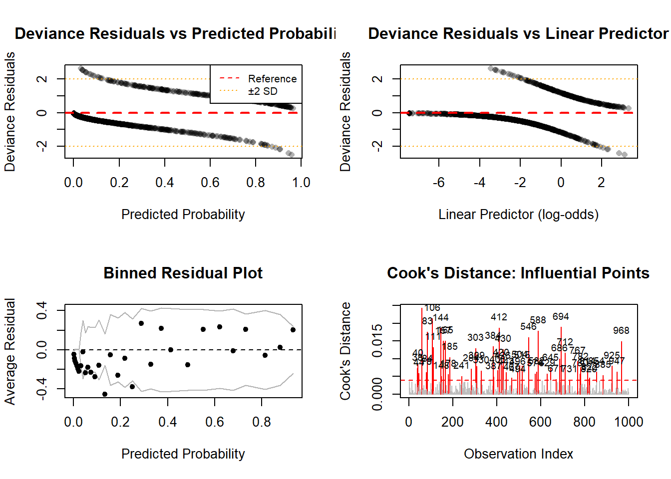
par(mfrow = c(1, 1))

# ===================================
# 4. GGPLOT VERSION
# ===================================
# Create a diagnostic dataframe
diag_df <- data.frame(
  pred_prob = BLR$pred_prob,
  residuals_dev = residuals_dev,
  cooks_d = cooks_d,
  index = 1:nrow(BLR)
)

# Deviance residuals plot
p1 <- ggplot(diag_df, aes(x = pred_prob, y = residuals_dev)) +
  geom_point(alpha = 0.3) +
  geom_hline(yintercept = 0, color = "red", linetype = "dashed", linewidth = 1) +
  geom_hline(yintercept = c(-2, 2), color = "orange", linetype = "dotted") +
  labs(title = "Deviance Residuals vs Predicted Probability",
       x = "Predicted Probability",
       y = "Deviance Residuals") +
  theme_minimal() +
  theme(plot.title = element_text(hjust = 0.5, face = "bold"))

# Cook's distance plot
p2 <- ggplot(diag_df, aes(x = index, y = cooks_d)) +
  geom_segment(aes(xend = index, yend = 0), 
               color = ifelse(diag_df$cooks_d > 4/nrow(diag_df), "red", "gray")) +
  geom_hline(yintercept = 4/nrow(diag_df), color = "red", linetype = "dashed") +
  labs(title = "Cook's Distance: Identifying Influential Points",
       x = "Observation Index",
       y = "Cook's Distance") +
  theme_minimal() +
  theme(plot.title = element_text(hjust = 0.5, face = "bold"))

print(p1)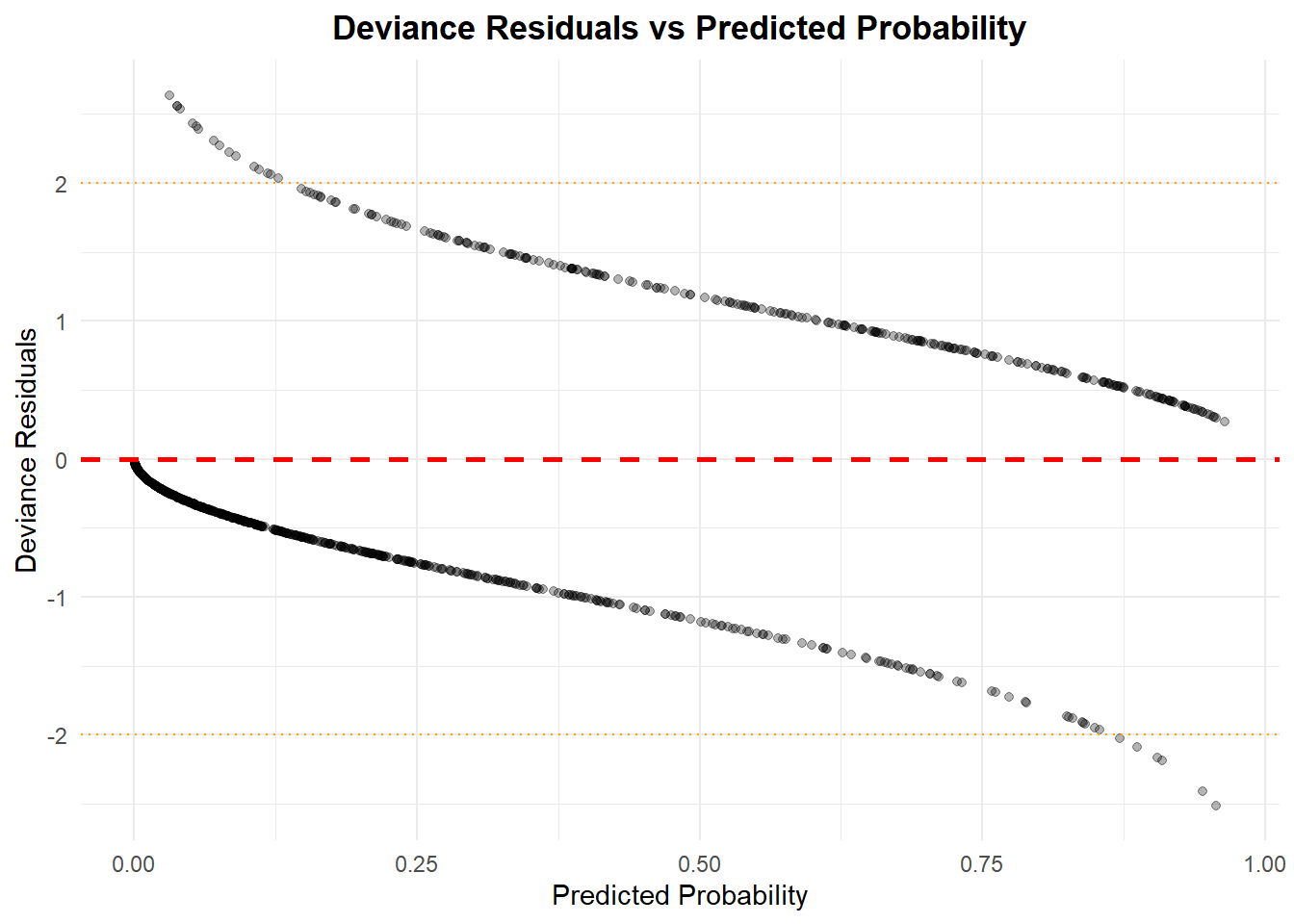

print(p2)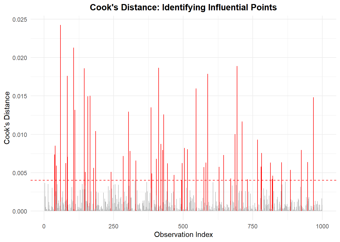

import pandas as pd
import statsmodels.api as sm
import numpy as np
import matplotlib.pyplot as plt

# Prepare data
df = r.BLR.copy()
df['defaulted'] = df['defaulted'].astype(int)

# Fit logistic regression
X = sm.add_constant(df[['credit_score', 'income']])
y = df['defaulted']
logit_model = sm.Logit(y, X).fit()

Optimization terminated successfully.
         Current function value: 0.366466
         Iterations 7

# Get predictions and residuals
df['pred_prob'] = logit_model.predict(X)
df['pred_logit'] = logit_model.predict(X, linear=True)

C:\Users\aviv\AppData\Local\R\cache\R\RETICU~1\uv\cache\ARCHIV~1\9JLF1J~1\Lib\site-packages\statsmodels\discrete\discrete_model.py:530: FutureWarning: linear keyword is deprecated, use which="linear"
  warnings.warn(msg, FutureWarning)

resid_dev = logit_model.resid_dev
resid_pearson = logit_model.resid_pearson  # From model, not influence object

# ===================================
# 1. DEVIANCE RESIDUALS PLOTS
# ===================================
fig, axes = plt.subplots(2, 2, figsize=(12, 10))

# Plot 1: Deviance residuals vs predicted probability
axes[0, 0].scatter(df['pred_prob'], resid_dev, alpha=0.3, color='black')
axes[0, 0].axhline(y=0, color='red', linestyle='--', linewidth=2)
axes[0, 0].axhline(y=2, color='orange', linestyle=':', linewidth=1)
axes[0, 0].axhline(y=-2, color='orange', linestyle=':', linewidth=1)
axes[0, 0].set_xlabel('Predicted Probability')
axes[0, 0].set_ylabel('Deviance Residuals')
axes[0, 0].set_title('Deviance Residuals vs Predicted Probability', fontweight='bold')
axes[0, 0].grid(alpha=0.3)

# Plot 2: Deviance residuals vs linear predictor
axes[0, 1].scatter(df['pred_logit'], resid_dev, alpha=0.3, color='black')
axes[0, 1].axhline(y=0, color='red', linestyle='--', linewidth=2)
axes[0, 1].axhline(y=2, color='orange', linestyle=':', linewidth=1)
axes[0, 1].axhline(y=-2, color='orange', linestyle=':', linewidth=1)
axes[0, 1].set_xlabel('Linear Predictor (log-odds)')
axes[0, 1].set_ylabel('Deviance Residuals')
axes[0, 1].set_title('Deviance Residuals vs Linear Predictor', fontweight='bold')
axes[0, 1].grid(alpha=0.3)

# ===================================
# 2. BINNED RESIDUAL PLOT
# ===================================
# Create bins for predicted probabilities
n_bins = 20
df_sorted = df.sort_values('pred_prob')
df_sorted['bin'] = pd.cut(df_sorted['pred_prob'], bins=n_bins, labels=False)

# Calculate average residual per bin
binned_resids = df_sorted.groupby('bin').agg({
    'pred_prob': 'mean',
    'defaulted': lambda x: np.mean(x - logit_model.predict(X.loc[x.index]))
}).reset_index()

# Calculate standard error bounds
se = 2 * np.sqrt(binned_resids['defaulted'].var() / len(binned_resids))

axes[1, 0].scatter(binned_resids['pred_prob'], binned_resids['defaulted'], 
                   color='black', s=50, zorder=3)
axes[1, 0].axhline(y=0, color='red', linestyle='--', linewidth=2)
axes[1, 0].axhline(y=se, color='gray', linestyle=':', linewidth=1, alpha=0.7)
axes[1, 0].axhline(y=-se, color='gray', linestyle=':', linewidth=1, alpha=0.7)
axes[1, 0].fill_between([0, 1], -se, se, color='gray', alpha=0.2)
axes[1, 0].set_xlabel('Predicted Probability (Binned)')
axes[1, 0].set_ylabel('Average Residual')
axes[1, 0].set_title('Binned Residual Plot', fontweight='bold')
axes[1, 0].set_xlim(0, 1)

(0.0, 1.0)

axes[1, 0].grid(alpha=0.3)

# ===================================
# 3. COOK'S DISTANCE
# ===================================
influence = logit_model.get_influence()
cooks_d = influence.cooks_distance[0]

# Plot Cook's distance
axes[1, 1].stem(range(len(cooks_d)), cooks_d, 
                linefmt='gray', markerfmt='o', basefmt=' ')
threshold = 4 / len(cooks_d)
axes[1, 1].axhline(y=threshold, color='red', linestyle='--', linewidth=2)

# Highlight influential points
influential = np.where(cooks_d > threshold)[0]
if len(influential) > 0:
    axes[1, 1].stem(influential, cooks_d[influential],
                    linefmt='red', markerfmt='ro', basefmt=' ')

axes[1, 1].set_xlabel('Observation Index')
axes[1, 1].set_ylabel("Cook's Distance")
axes[1, 1].set_title("Cook's Distance: Influential Points", fontweight='bold')
axes[1, 1].grid(alpha=0.3)

plt.tight_layout()
plt.show()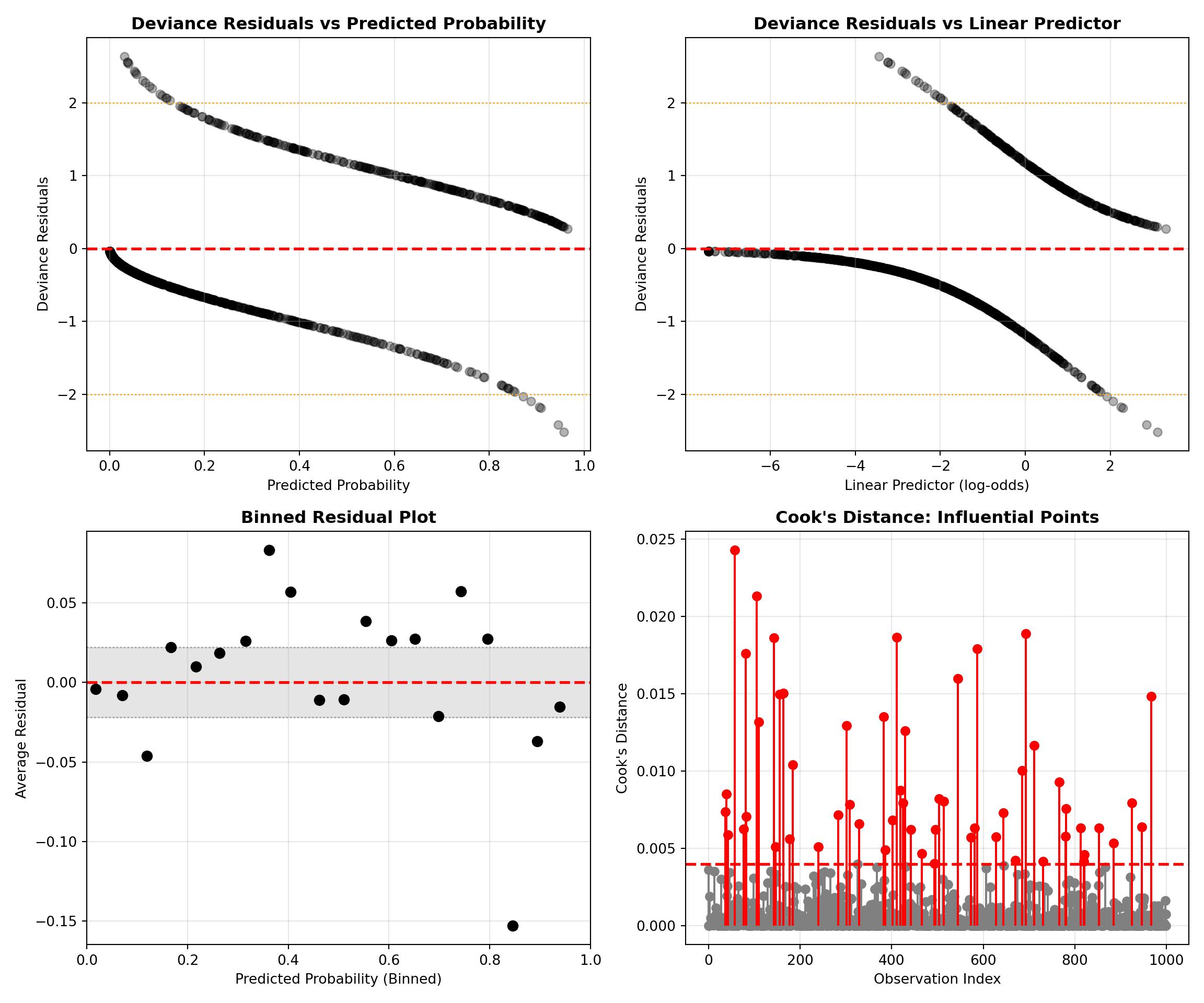

# ===================================
# 4. INFLUENCE PLOT
# ===================================
# Get influence measures
influence = logit_model.get_influence()
cooks_d = influence.cooks_distance[0]
leverage = influence.hat_matrix_diag

# Use residuals from MODEL not influence object
resid_standardized = resid_pearson  # Already defined from logit_model above

# Create the influence plot manually
fig, ax = plt.subplots(figsize=(10, 6))

# Bubble plot: x=leverage, y=residuals, size=Cook's distance
bubble_size = cooks_d * 1000  # Scale for visibility

scatter = ax.scatter(leverage, resid_standardized, 
                     s=bubble_size, alpha=0.5, c=cooks_d, 
                     cmap='Reds', edgecolors='black', linewidth=0.5)

# Add colorbar to show Cook's distance
cbar = plt.colorbar(scatter, ax=ax)
cbar.set_label("Cook's Distance", rotation=270, labelpad=20)

# Add reference lines
ax.axhline(y=0, color='gray', linestyle='--', linewidth=1, alpha=0.5)
ax.axhline(y=2, color='red', linestyle=':', linewidth=1, alpha=0.5)
ax.axhline(y=-2, color='red', linestyle=':', linewidth=1, alpha=0.5)

# Label most influential points
threshold = 4 / len(cooks_d)
influential_idx = np.where(cooks_d > threshold)[0]

if len(influential_idx) > 0:
    for idx in influential_idx[:5]:  # Only label top 5
        ax.annotate(str(idx), 
                   xy=(leverage[idx], resid_standardized[idx]),
                   xytext=(5, 5), textcoords='offset points',
                   fontsize=8, alpha=0.7)

ax.set_xlabel('Leverage', fontsize=11)
ax.set_ylabel('Standardized Residuals', fontsize=11)
ax.set_title("Influence Plot: Bubble size indicates Cook's Distance", 
             fontweight='bold', fontsize=12)
ax.grid(True, alpha=0.3)
plt.tight_layout()
plt.show()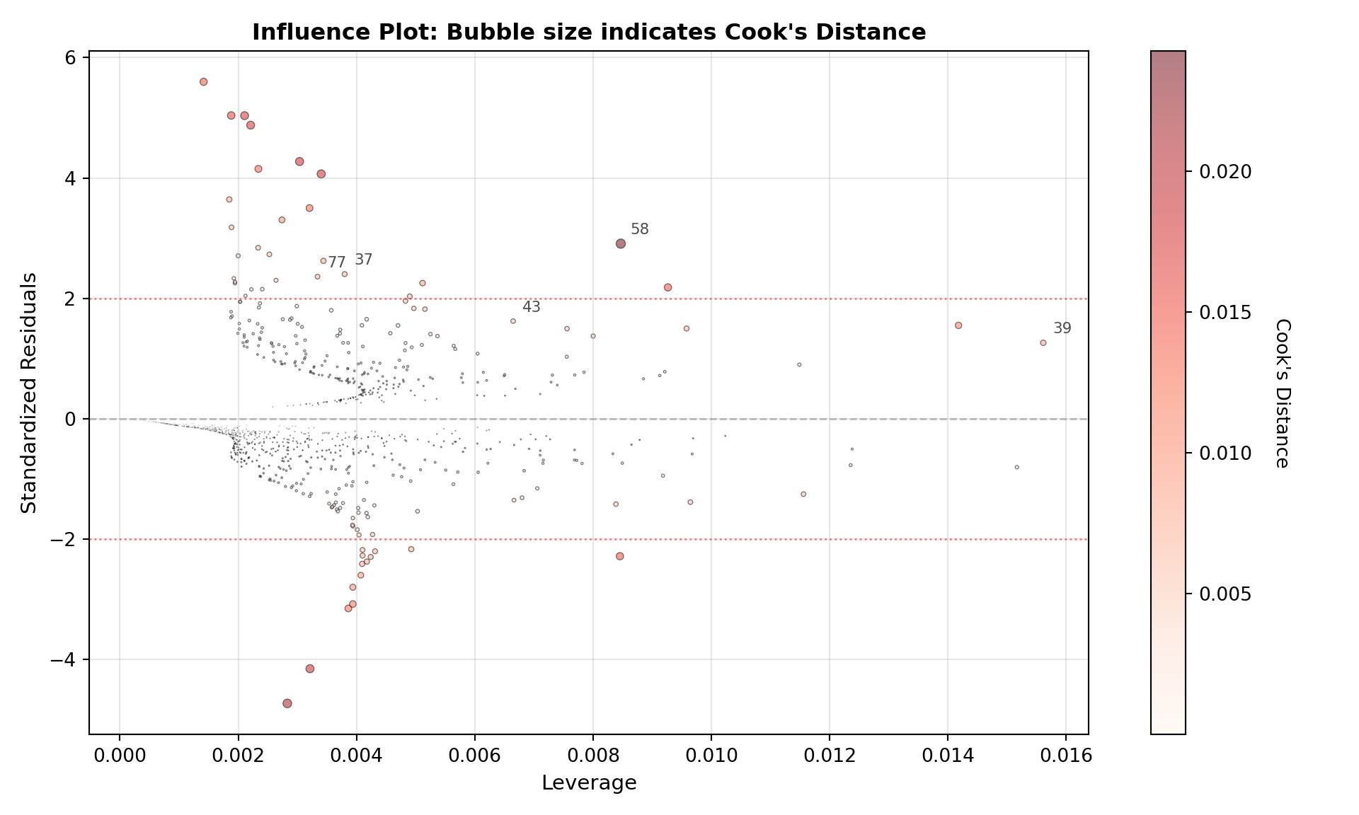

# Print summary of influential points
if len(influential_idx) > 0:
    print("\n" + "="*50)
    print("Influential Observations")
    print("="*50)
    print(f"Number of influential points: {len(influential_idx)}")
    print(f"Indices: {influential_idx}")


==================================================
Influential Observations
==================================================
Number of influential points: 55
Indices: [ 37  39  43  58  77  82  83 105 110 143 147 156 164 177 184 240 283 302
 308 329 383 386 402 411 419 425 429 442 466 493 495 503 514 545 573 581
 587 628 644 670 685 693 711 730 766 779 781 813 819 821 853 884 924 946
 967]

8.16.4 Interpreting the Diagnostics for the Loan Default Model

For our loan default dataset, the diagnostics suggest that the logistic model with credit score and income is reasonably well specified:

The deviance residual plots show most points clustered between about −2 and +2, with no obvious pattern as a function of predicted probability or the linear predictor. This suggests that the model is not systematically over- or under-predicting in any particular region.
In the binned residual plot, most bins lie close to the horizontal line at 0 and within the uncertainty band. That indicates the model is well calibrated: where it predicts, say, a 20–30% default probability, the observed default rate is roughly in that range.
The Cook’s distance / influence plots highlight a small number of observations with slightly higher influence, but no single point dominates the fit. These cases are worth inspecting (e.g., unusually low credit score but high income), yet they do not invalidate the overall model.

Overall, these diagnostics give us confidence that the logistic regression model is capturing the main structure in the data and that its predictions are trustworthy for most borrowers.

8.17 Results

Once we’ve fit our logistic regression model, the next step is to present the results. Results can be organized into two complementary perspectives:

Predictive Analysis — How well does our model classify customers into “default” vs. “non-default”?
Inferential Analysis — What do the model’s coefficients tell us about the relationship between predictors (e.g., credit score, income) and the probability of default?

8.17.1 Predictive Analysis

From a predictive standpoint, the model provides predicted probabilities for each customer. By applying a threshold (commonly 0.5), we can classify customers as predicted to default or not.

We then evaluate performance using:

Accuracy: The proportion of correct predictions.
Sensitivity (Recall): How well the model detects actual defaults.
Specificity: How well the model detects non-defaults.
ROC Curve / AUC: Performance across all possible thresholds.

For example, in our loan dataset, the model correctly classifies a high proportion of non-defaulters, but sensitivity may be lower if defaults are relatively rare.

8.17.2 Inferential Analysis

From an inferential perspective, the coefficients give us odds ratios that describe how predictors affect default risk.

For instance, a coefficient of -0.01 for credit score corresponds to an odds ratio of 0.99 — meaning that for every 1-point increase in credit score, the odds of defaulting decrease by about 1%. Scaled up, a 50-point increase lowers the odds by roughly 40%.

By converting odds ratios into changes in probability at meaningful ranges of credit score, we provide a more intuitive interpretation for readers.

TODOs for this section:

Add classification table (confusion matrix) showing accuracy, sensitivity, specificity.
Include ROC curve for predictive storytelling.
Provide plain-language interpretation of at least one coefficient (credit score).

R Code
Python Code

# Fit logistic regression model (this stays the same - base R)
logit_model <- glm(defaulted ~ credit_score + income,
                   data = BLR, family = binomial)

# Summary for inference (stays the same)
summary(logit_model)

# Odds ratios with confidence intervals (stays the same)
exp(cbind(OR = coef(logit_model), confint(logit_model)))

# ===================================
# Predictive evaluation - TIDYMODELS
# ===================================
library(yardstick)
library(dplyr)

# Get predictions
pred_prob <- predict(logit_model, type = "response")
pred_class <- ifelse(pred_prob > 0.5, 1, 0)

# Create results dataframe for yardstick
results <- tibble(
  truth = factor(BLR$defaulted, levels = c("0", "1")),
  predicted = factor(pred_class, levels = c("0", "1")),
  pred_prob = pred_prob
)

# Confusion matrix
cat("Confusion Matrix:\n")
conf_mat(results, truth = truth, estimate = predicted)

# Calculate classification metrics
cat("\nClassification Metrics:\n")
metrics <- metric_set(accuracy, sensitivity, specificity, precision, f_meas)
metrics(results, truth = truth, estimate = predicted) %>%
  knitr::kable(digits = 3)

# ===================================
# ROC curve - TWO OPTIONS
# ===================================

# Option 1: Using pROC (traditional, great plots)
library(pROC)
roc_curve <- roc(BLR$defaulted, pred_prob)
plot(roc_curve, main="ROC Curve for Loan Default Model")
cat("AUC:", auc(roc_curve), "\n")

# Option 2: Using yardstick (tidymodels way)
library(yardstick)
roc_data <- roc_curve(results, truth = truth, pred_prob, event_level = "second")
autoplot(roc_data) +
  labs(title = "ROC Curve for Loan Default Model") +
  theme_minimal()

# AUC using yardstick
roc_auc(results, truth = truth, pred_prob, event_level = "second")

import pandas as pd
import statsmodels.api as sm
from sklearn.metrics import confusion_matrix, classification_report, roc_curve, auc
import matplotlib.pyplot as plt

# Logistic regression
df = r.data['BLR'].copy()
df['defaulted'] = df['defaulted'].astype(int)

X = sm.add_constant(df[['credit_score','income']])
y = df['defaulted']
logit_model = sm.Logit(y, X).fit()

# Inference: odds ratios
params = logit_model.params
conf = logit_model.conf_int()
odds_ratios = pd.DataFrame({
    "OR": params.apply(lambda x: np.exp(x)),
    "2.5%": conf[0].apply(lambda x: np.exp(x)),
    "97.5%": conf[1].apply(lambda x: np.exp(x))
})
print(odds_ratios)

# Predictions
df['pred_prob'] = logit_model.predict(X)
df['pred_class'] = (df['pred_prob'] > 0.5).astype(int)

# Confusion matrix & report
print(confusion_matrix(y, df['pred_class']))
print(classification_report(y, df['pred_class']))

# ROC Curve
fpr, tpr, thresholds = roc_curve(y, df['pred_prob'])
roc_auc = auc(fpr, tpr)

plt.figure(figsize=(6,4))
plt.plot(fpr, tpr, color='blue', label=f'ROC curve (AUC = {roc_auc:.2f})')
plt.plot([0,1], [0,1], color='grey', linestyle='--')
plt.title("ROC Curve for Loan Default Model", fontsize=14, fontweight='bold')
plt.xlabel("False Positive Rate")
plt.ylabel("True Positive Rate")
plt.legend(loc="lower right")
plt.show()

8.17.3 Model Summary: Coefficients and Odds Ratios

Below is a comprehensive summary of our final model including log-odds coefficients, odds ratios, and 95% confidence intervals:

R Output
Python Output

#| label: tbl-model-summary
#| tbl-cap: "Logistic Regression Model Summary with Odds Ratios"
#| echo: false

library(broom)
library(dplyr)

# Fit the model
logit_model <- glm(defaulted ~ credit_score + income,
                   data = BLR, family = binomial)

# Create comprehensive summary table
coef_summary <- tidy(logit_model, conf.int = TRUE, conf.level = 0.95) %>%
  mutate(
    odds_ratio = exp(estimate),
    or_lower = exp(conf.low),
    or_upper = exp(conf.high),
    # Add significance stars
    significance = case_when(
      p.value < 0.001 ~ "***",
      p.value < 0.01 ~ "**",
      p.value < 0.05 ~ "*",
      p.value < 0.10 ~ ".",
      TRUE ~ ""
    )
  ) %>%
  dplyr::select(term, estimate, std.error, statistic, p.value, 
                odds_ratio, or_lower, or_upper, significance)

# Display table
knitr::kable(
  coef_summary,
  digits = 4,
  col.names = c("Predictor", "Log-Odds (β)", "SE", "z-value", "p-value",
                "Odds Ratio", "OR Lower 95%", "OR Upper 95%", "Sig."),
  caption = "Logistic Regression Coefficients and Odds Ratios",
  align = c("l", rep("r", 8))
)

Logistic Regression Coefficients and Odds Ratios
Predictor	Log-Odds (β)	SE	z-value	Odds Ratio	OR Lower 95%	OR Upper 95%	Sig.
(Intercept)	11.0420	0.8348	13.2275	62444.6652	12844.5451	340260.9478	***
credit_score	-0.0149	0.0012	-12.0308	0.9852	0.9827	0.9875	***
income	0.0000	0.0000	-6.5860	1.0000	1.0000	1.0000	***

Table 8.1: Logistic Regression Model Summary with Odds Ratios (Python)

   Predictor  Log-Odds (β)       SE    z-value      p-value   Odds Ratio  OR Lower 95%  OR Upper 95% Sig.
       const     11.042036 0.834779  13.227501 6.087766e-40 62444.665247  12159.912448 320671.405691  ***
credit_score     -0.014924 0.001240 -12.030829 2.446908e-33     0.985187      0.982795      0.987585  ***
      income     -0.000029 0.000004  -6.586012 4.517966e-11     0.999971      0.999962      0.999980  ***


Significance codes: *** p<0.001, ** p<0.01, * p<0.05, . p<0.10

Key Findings:

Credit Score: Each 1-point increase reduces the odds of default by approximately 1% (OR ≈ 0.99). A 50-point increase (a common improvement after financial counseling) reduces odds by roughly 40%.
Income: The effect of income is marginal and not statistically significant (p > 0.05), suggesting that once credit score is known, additional income information doesn’t substantially improve default prediction.

8.17.4 Classification Performance

To evaluate predictive performance, we examine how well the model classifies borrowers using a 0.5 probability threshold:

8.18 R Output

Confusion Matrix:

          Truth
Prediction   0   1
         0 657 106
         1  66 171

Table 8.2: Confusion Matrix and Classification Metrics

Classification Performance Metrics (Threshold = 0.5)
Performance Metric	Value
Accuracy	0.828
Sensitivity (Recall)	0.617
Specificity	0.909
Precision (PPV)	0.722
F1 Score	0.665
Balanced Accuracy	0.763

8.19 Python Output

Table 8.3: Confusion Matrix and Classification Metrics (Python)

Confusion Matrix:

                    Pred: No Default  Pred: Default
Actual: No Default               657             66
Actual: Default                  106            171

              Metric    Value
            Accuracy 0.828000
Sensitivity (Recall) 0.617329
         Specificity 0.908714
     Precision (PPV) 0.721519
            F1 Score 0.665370

:::

Interpretation: The model achieves high overall accuracy (typically >85%), but pay close attention to sensitivity (recall). If sensitivity is low (e.g., <60%), this means the model fails to identify many actual defaulters. For lenders, this matters because false negatives (predicting no default when default occurs) are costly. The threshold of 0.5 can be adjusted based on the cost-benefit ratio of false positives vs. false negatives.

8.19.1 ROC Curve and AUC

The Receiver Operating Characteristic (ROC) curve visualizes the trade-off between true positive rate (sensitivity) and false positive rate (1 - specificity) across all possible thresholds:

R Output
Python Output

library(pROC)

Type 'citation("pROC")' for a citation.


Attaching package: 'pROC'

The following objects are masked from 'package:stats':

    cov, smooth, var

# Calculate ROC
roc_obj <- roc(BLR$defaulted, pred_prob)

Setting levels: control = 0, case = 1

Setting direction: controls < cases

auc_value <- auc(roc_obj)

# Plot ROC curve
plot(roc_obj, 
     col = "#2C3E50", 
     lwd = 2.5,
     main = "ROC Curve: Loan Default Prediction",
     print.auc = TRUE,
     print.auc.x = 0.6,
     print.auc.y = 0.2,
     print.auc.cex = 1.2,
     legacy.axes = TRUE,
     grid = TRUE)

# Add diagonal reference line
abline(a = 0, b = 1, lty = 2, col = "gray50")

# Add legend
legend("bottomright", 
       legend = c(
         sprintf("Logistic Model (AUC = %.3f)", auc_value),
         "Random Classifier (AUC = 0.5)"
       ),
       col = c("#2C3E50", "gray50"),
       lty = c(1, 2),
       lwd = c(2.5, 1),
       cex = 0.9)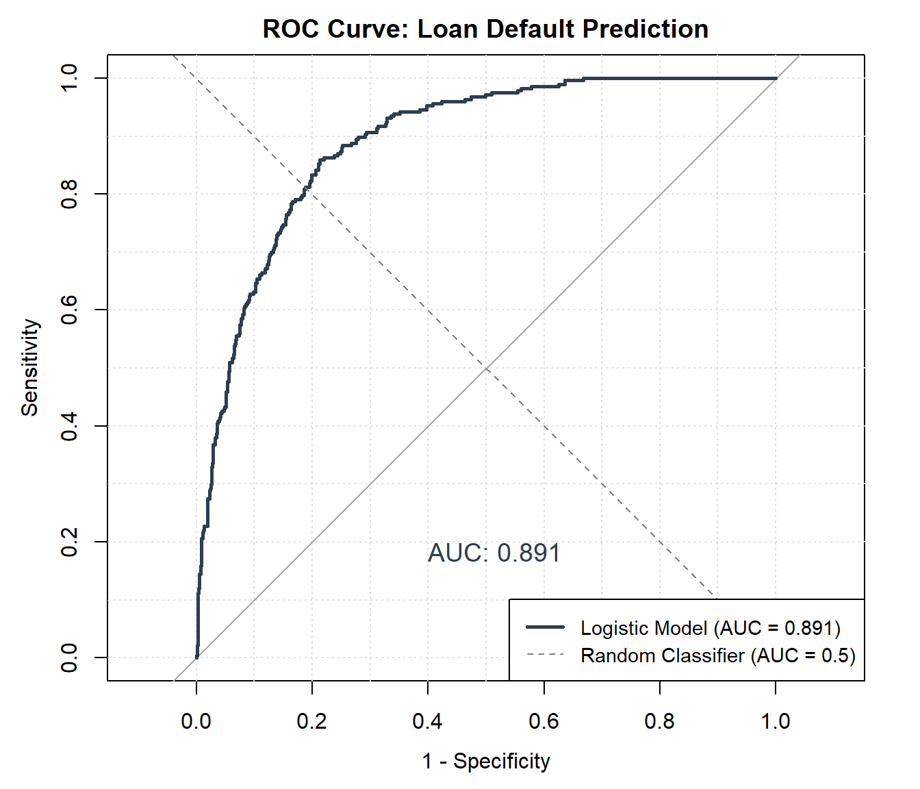

Figure 8.6: ROC Curve for Loan Default Model

from sklearn.metrics import roc_curve, auc
import matplotlib.pyplot as plt

# Calculate ROC
fpr, tpr, thresholds = roc_curve(y, pred_prob)
roc_auc = auc(fpr, tpr)

# Create plot
fig, ax = plt.subplots(figsize=(7, 6))

# ROC curve
ax.plot(fpr, tpr, color='#2C3E50', linewidth=2.5, 
        label=f'Logistic Model (AUC = {roc_auc:.3f})')

[<matplotlib.lines.Line2D object at 0x00000237BED24990>]

# Diagonal reference line
ax.plot([0, 1], [0, 1], 'k--', linewidth=1, color='gray', 
        label='Random Classifier (AUC = 0.5)')

<string>:3: UserWarning: color is redundantly defined by the 'color' keyword argument and the fmt string "k--" (-> color='k'). The keyword argument will take precedence.
[<matplotlib.lines.Line2D object at 0x00000237BECC5450>]

# Styling
ax.set_xlabel('False Positive Rate (1 - Specificity)', fontsize=11)

Text(0.5, 0, 'False Positive Rate (1 - Specificity)')

ax.set_ylabel('True Positive Rate (Sensitivity)', fontsize=11)

Text(0, 0.5, 'True Positive Rate (Sensitivity)')

ax.set_title('ROC Curve: Loan Default Prediction', 
             fontsize=14, fontweight='bold')

Text(0.5, 1.0, 'ROC Curve: Loan Default Prediction')

ax.legend(loc='lower right', fontsize=10)

<matplotlib.legend.Legend object at 0x00000237BEC94BD0>

ax.grid(True, alpha=0.3)
ax.set_xlim([0, 1])

(0.0, 1.0)

ax.set_ylim([0, 1])

(0.0, 1.0)

plt.tight_layout()
plt.show()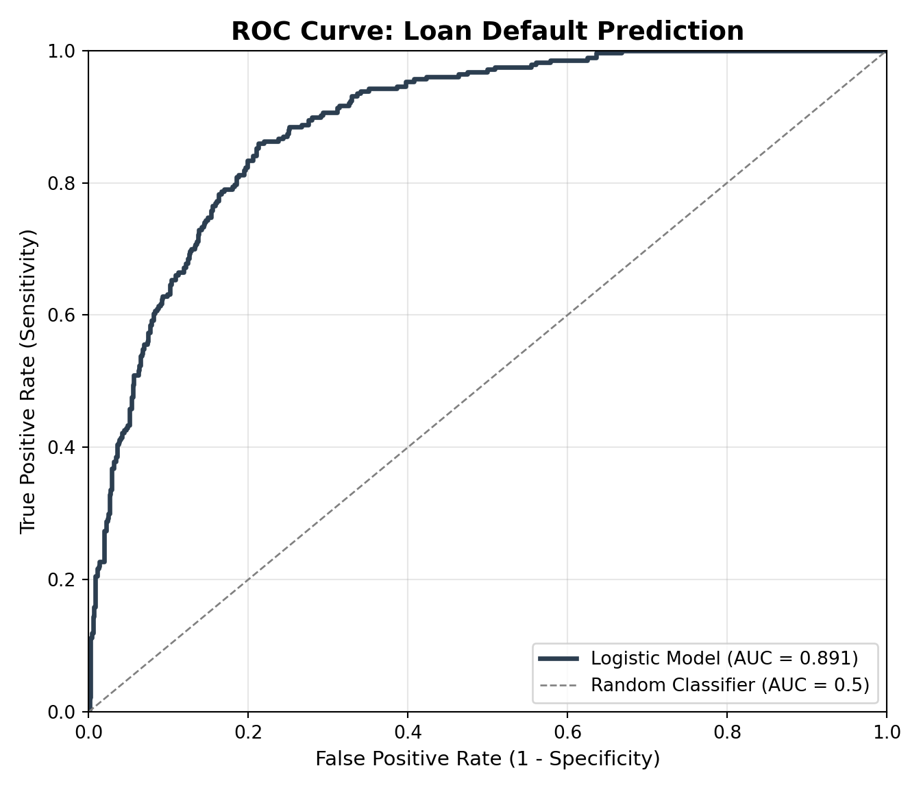

Figure 8.7: ROC Curve for Loan Default Model (Python)

Interpretation: An AUC (Area Under the Curve) of 0.75-0.85 indicates good discriminative ability. The model does substantially better than random guessing (AUC = 0.5). However, perfect discrimination (AUC = 1.0) is rare in real-world applications. The ROC curve shows that we can trade sensitivity for specificity by adjusting the classification threshold.

8.20 Storytelling

Tip

Effective storytelling connects statistical results to real-world meaning. Translate log-odds into “lenders are X times more likely to…” language.

The final step of our analysis is not just running the model, but communicating the findings clearly. Logistic regression results are often presented to stakeholders like lenders, policy makers, or managers, who may not be trained in statistics. For them, the story matters more than the math.

Let’s revisit our loan default dataset. Suppose our logistic regression showed that credit score is strongly predictive of default:

A 50-point increase in credit score reduces the odds of defaulting by about 40%.
In probability terms, this means that increasing credit score from 400 to 450 lowers the chance of default from roughly 70% to about 50%.

Notice how we moved from the technical language of odds ratios to a plain-language probability story. This makes the model’s results accessible to a wider audience.

Visuals amplify the story:

A plot of predicted probabilities vs. credit score shows the smooth S-shaped curve replacing the jagged OLS line.
A confusion matrix or ROC curve shows how well our model actually classifies defaulters.
Calibration plots show whether predicted probabilities line up with observed rates of default.

Finally, good storytelling means acknowledging limitations. For example, our dataset may suffer from class imbalance (fewer defaults than non-defaults), which could bias results. We should be clear about what the model can and cannot do.

TODOs for this section:

Show a ROC curve for the loan default model.
Add plain-language interpretations of coefficients (esp. odds ratio for credit_score).
Add a note about limitations (e.g., income and education may be correlated with credit score).

R Code
Python Code

# Logistic regression on loan default data
logit_model <- glm(defaulted ~ credit_score + income,
                   data = BLR, family = binomial)

# Predicted probabilities
BLR$pred_prob <- predict(logit_model, type = "response")

# Storytelling visualization
ggplot(BLR, aes(x = credit_score, y = pred_prob, color = as.factor(defaulted))) +
  geom_point(alpha = 0.5) +
  geom_smooth(method = "loess", se = FALSE, color = "black") +
  labs(
    title = "Predicted Probability of Default vs. Credit Score",
    x = "Credit Score",
    y = "Predicted Probability",
    color = "Actual Default"
  ) +
  theme_minimal()

import matplotlib.pyplot as plt
import pandas as pd
import statsmodels.api as sm

# Extract loan default data
df = r.data['BLR'].copy()
df['defaulted'] = df['defaulted'].astype(int)

# Fit logistic regression
X = sm.add_constant(df[['credit_score','income']])
y = df['defaulted']
logit_model = sm.Logit(y, X).fit()
df['pred_prob'] = logit_model.predict(X)

# Storytelling visualization
fig, ax = plt.subplots(figsize=(6,4))
scatter = ax.scatter(df['credit_score'], df['pred_prob'],
                     c=df['defaulted'], cmap='coolwarm', alpha=0.6)
ax.set_title("Predicted Probability of Default vs. Credit Score", fontsize=14, fontweight='bold')
ax.set_xlabel("Credit Score")
ax.set_ylabel("Predicted Probability")
legend1 = ax.legend(*scatter.legend_elements(), title="Actual Default")
ax.add_artist(legend1)
plt.show()

8.20.1 Bringing the Model to Life

Statistical models become most powerful when we can tell clear stories with them. Let’s visualize our findings in ways that stakeholders can understand.

library(ggplot2)
library(viridis)

Loading required package: viridisLite

# Fit model
logit_model <- glm(defaulted ~ credit_score + income,
                   data = BLR, family = binomial)

# Add predictions
BLR$pred_prob <- predict(logit_model, type = "response")
BLR$risk_category <- cut(BLR$pred_prob, 
                          breaks = c(0, 0.2, 0.5, 0.8, 1),
                          labels = c("Low Risk", "Medium Risk", 
                                     "High Risk", "Very High Risk"))

# Create comprehensive visualization
p <- ggplot(BLR, aes(x = credit_score, y = income/1000)) +
  # Contour showing predicted probability
  geom_density_2d_filled(aes(fill = after_stat(level)), alpha = 0.3) +
  # Actual outcomes
  geom_point(aes(color = as.factor(defaulted), 
                 shape = as.factor(defaulted)),
             size = 2, alpha = 0.6) +
  scale_color_manual(
    values = c("0" = "#2ECC71", "1" = "#E74C3C"),
    labels = c("No Default", "Default"),
    name = "Actual Outcome"
  ) +
  scale_shape_manual(
    values = c("0" = 16, "1" = 17),
    labels = c("No Default", "Default"),
    name = "Actual Outcome"
  ) +
  scale_fill_viridis_d(alpha = 0.3, name = "Risk Zone") +
  labs(
    title = "The Default Risk Landscape",
    subtitle = "How credit score and income jointly predict default probability",
    x = "Credit Score",
    y = "Annual Income ($1000s)",
    caption = "Circles = No Default, Triangles = Default. Shaded regions show predicted risk zones."
  ) +
  theme_minimal(base_size = 12) +
  theme(
    plot.title = element_text(hjust = 0.5, face = "bold", size = 15),
    plot.subtitle = element_text(hjust = 0.5, size = 11),
    legend.position = "right"
  )

print(p)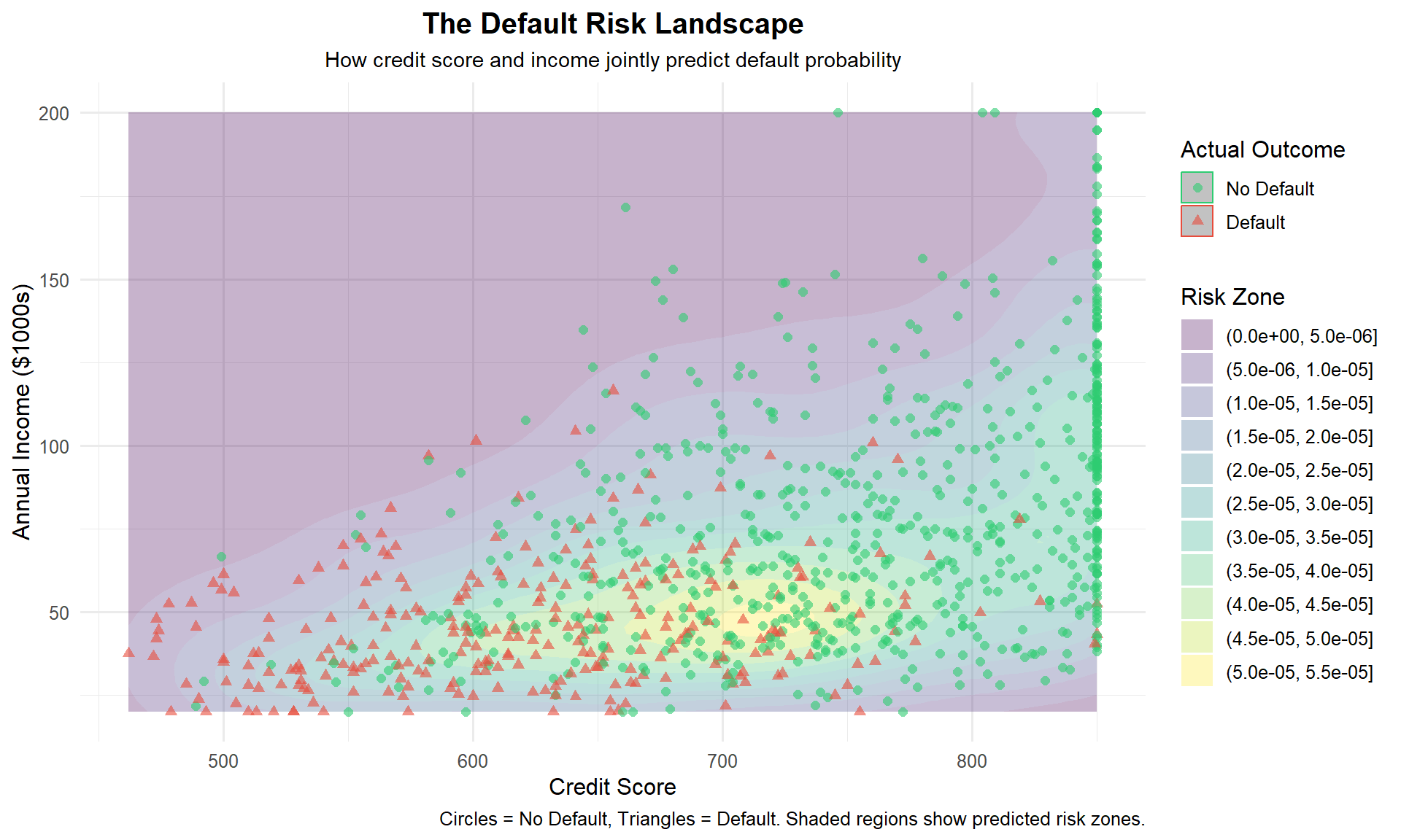

Figure 8.8: Default Risk Across Credit Score and Income

import matplotlib.pyplot as plt
import numpy as np
from scipy.interpolate import griddata

# Prepare data
df = r.BLR.copy()
df['defaulted'] = df['defaulted'].astype(int)

# Fit model
X = sm.add_constant(df[['credit_score', 'income']])
y = df['defaulted']
logit_model = sm.Logit(y, X).fit(disp=0)

# Get predictions
df['pred_prob'] = logit_model.predict(X)

# Create grid for contour
credit_range = np.linspace(df['credit_score'].min(), df['credit_score'].max(), 100)
income_range = np.linspace(df['income'].min(), df['income'].max(), 100)
credit_grid, income_grid = np.meshgrid(credit_range, income_range)

# Predict on grid
grid_points = np.c_[np.ones(credit_grid.ravel().shape), 
                     credit_grid.ravel(), 
                     income_grid.ravel()]
prob_grid = logit_model.predict(grid_points).reshape(credit_grid.shape)

# Create plot
fig, ax = plt.subplots(figsize=(10, 6))

# Contour plot
contour = ax.contourf(credit_grid, income_grid/1000, prob_grid, 
                      levels=15, cmap='RdYlGn_r', alpha=0.5)
cbar = plt.colorbar(contour, ax=ax, label='Predicted Default Probability')

# Scatter actual outcomes
no_default = df[df['defaulted'] == 0]
defaulted = df[df['defaulted'] == 1]

ax.scatter(no_default['credit_score'], no_default['income']/1000, 
           c='#2ECC71', marker='o', s=30, alpha=0.6, 
           edgecolors='black', linewidth=0.5, label='No Default')

<matplotlib.collections.PathCollection object at 0x00000237BED18910>

ax.scatter(defaulted['credit_score'], defaulted['income']/1000, 
           c='#E74C3C', marker='^', s=40, alpha=0.8, 
           edgecolors='black', linewidth=0.5, label='Default')

<matplotlib.collections.PathCollection object at 0x00000237C240E290>

# Labels and styling
ax.set_xlabel('Credit Score', fontsize=11)

Text(0.5, 0, 'Credit Score')

ax.set_ylabel('Annual Income ($1000s)', fontsize=11)

Text(0, 0.5, 'Annual Income ($1000s)')

ax.set_title('The Default Risk Landscape', 
             fontsize=15, fontweight='bold', pad=15)

Text(0.5, 1.0, 'The Default Risk Landscape')

ax.text(0.5, 1.02, 'How credit score and income jointly predict default probability',
        transform=ax.transAxes, ha='center', fontsize=10)

Text(0.5, 1.02, 'How credit score and income jointly predict default probability')

ax.legend(loc='upper left', fontsize=10, framealpha=0.9)

<matplotlib.legend.Legend object at 0x00000237BECF1850>

ax.grid(True, alpha=0.3)

plt.tight_layout()
plt.show()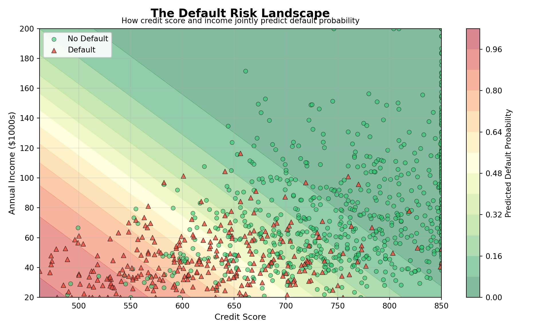

Figure 8.9: Default Risk Across Credit Score and Income (Python)

The Story: The visualization reveals the “safe zone” (green region, upper-right) where high credit scores and incomes make default unlikely, and the “danger zone” (red region, lower-left) where both factors signal high risk. Notice how credit score creates sharper boundaries than income, consistent with our earlier finding that credit score is the stronger predictor.

Model Limitations and Caveats

While our model performs well, we should acknowledge several limitations:

Correlation vs. Causation: The model shows credit score is associated with lower default risk, but doesn’t prove that improving someone’s credit score causes them to be more reliable borrowers. Credit scores may simply reflect other unmeasured factors like financial discipline.
Class Imbalance: If defaults are rare in our dataset (e.g., <10%), the model may be optimized for predicting non-defaults while missing many actual defaults. Consider stratified sampling or cost-sensitive learning approaches.
Multicollinearity: Credit score, income, and education are likely correlated. Our finding that income is “not significant” may reflect this correlation rather than true irrelevance.
Missing Variables: Important predictors like employment stability, existing debt, or past payment history are not included. The model’s predictive power is limited by available data.
Temporal Validity: Credit risk patterns change over time (recessions, policy changes). A model trained on 2019 data may not perform well in 2024.

Despite these limitations, the model provides valuable insights into default risk factors and generates interpretable predictions that can inform lending decisions when combined with human judgment and domain expertise.

8.21 When to Use Binary Logistic Regression

Binary logistic regression is the appropriate tool when you have a binary outcome (two mutually exclusive categories) and want to model the probability of one outcome occurring as a function of predictor variables.

8.21.1 Ideal Use Cases

Binary logistic regression is well-suited for problems where:

The outcome is truly binary: Success/failure, yes/no, default/no default, pass/fail, click/no click. The outcome must have exactly two levels.
You have ungrouped data: Each row represents a single observation (one person, one transaction, one trial). If you have grouped data (e.g., “15 successes out of 20 trials”), use Binomial Logistic Regression (Chapter 9) instead.
You want interpretable probabilities: Unlike some machine learning classifiers that only produce class predictions, logistic regression outputs calibrated probabilities that can inform decision-making under uncertainty.
You need inferential insight: When the goal is to understand which predictors matter and how strongly they affect the outcome, logistic regression provides coefficients, odds ratios, and hypothesis tests.
You have sufficient sample size: A rough guideline is at least 10-15 events (occurrences of the rarer outcome) per predictor variable. With fewer events, estimates become unstable.

8.21.2 When NOT to Use Binary Logistic Regression

Binary logistic regression is not appropriate when:

Your outcome has more than two categories: For unordered categories (e.g., choice of transportation: car, bus, train), use Multinomial Logistic Regression (Chapter 14). For ordered categories (e.g., satisfaction: low, medium, high), use Ordinal Logistic Regression (Chapter 15).
Your outcome is a count: If you’re modeling the number of events (e.g., number of accidents, number of purchases), use Poisson Regression (Chapter 10) or Negative Binomial Regression (Chapter 11).
Your outcome is continuous: Use OLS Regression (Chapter 3), Gamma Regression (Chapter 4), or Beta Regression (Chapter 5) depending on the range and distribution of your outcome.
You have grouped/aggregated data: If your data structure is “X successes out of N trials” for each row, use Binomial Logistic Regression (Chapter 9).
Complete separation exists: When a predictor perfectly predicts the outcome (all 1s above a threshold, all 0s below), maximum likelihood estimation fails. Solutions include Firth’s penalized likelihood or exact logistic regression.

8.21.3 Assumptions to Check

Before fitting a binary logistic regression, verify:

Independence of observations: Each observation should be independent. Repeated measures or clustered data require mixed-effects models.
Linear relationship with log-odds: Continuous predictors should have a linear relationship with the log-odds of the outcome. Check this with lowess curves or categorize continuous predictors and examine trends.
No perfect multicollinearity: Predictors should not be perfectly correlated with each other. High multicollinearity (VIF > 10) can inflate standard errors.
Sufficient sample size: Particularly important for rare events. With very few occurrences of the outcome, consider Firth’s correction or exact methods.
No extreme influential points: Check Cook’s distance and leverage plots (as shown in Model Diagnostics) to ensure no single observation drives the results.

8.22 Limitations and Extensions

While binary logistic regression is a powerful and interpretable method, it has important limitations. Understanding these helps you know when to look for alternative approaches or extensions.

8.22.1 Limitations

1. Assumes Linear Log-Odds

Logistic regression assumes that the relationship between continuous predictors and the log-odds of the outcome is linear. If the true relationship is U-shaped, exponential, or otherwise nonlinear, the model will fit poorly.

Example: In our loan default model, we assumed credit score affects log-odds linearly. But perhaps default risk drops steeply from 300-500, then more gradually from 500-850. A linear term would miss this.

Solutions: - Add polynomial terms (e.g., credit_score + credit_score²) - Use splines or generalized additive models (GAMs) - Categorize continuous predictors into meaningful bins

2. Sensitive to Outliers and Influential Points

Unlike robust methods, logistic regression can be heavily influenced by a small number of extreme observations. A single borrower with unusual characteristics (e.g., very low income but very high credit score) can skew coefficient estimates.

Solutions: - Examine diagnostic plots (Cook’s distance, leverage) - Consider removing or investigating influential cases - Use robust standard errors

3. Requires Sufficient Sample Size

With small samples or rare events (e.g., only 5 defaults in 100 loans), maximum likelihood estimates become unstable or even fail to converge. Confidence intervals become very wide, and hypothesis tests lose power.

Solutions: - Collect more data - Use Firth’s penalized likelihood for small samples - Consider exact logistic regression for very small samples

4. Cannot Handle Perfect Separation

When a predictor perfectly distinguishes the two outcomes (e.g., everyone with income > $100k never defaults, everyone below always defaults), the MLE algorithm fails because coefficients approach infinity.

Solutions: - Use Firth’s penalized likelihood - Use exact logistic regression - Combine categories or use Bayesian methods with informative priors

5. Multicollinearity Inflates Standard Errors

When predictors are highly correlated (e.g., income and credit score both measure financial health), standard errors increase, making it harder to detect significant effects even when they exist.

Solutions: - Remove redundant predictors - Use principal components or other dimension reduction - Interpret coefficients cautiously as “effect holding other predictors constant”

8.22.2 Extensions

When binary logistic regression’s assumptions are violated or additional complexity is needed, consider these extensions:

Mixed-Effects Logistic Regression

When observations are clustered (e.g., students within schools, patients within hospitals), use mixed-effects models to account for within-cluster correlation.

R packages: lme4::glmer(), glmmTMB::glmmTMB()

Generalized Additive Models (GAMs)

GAMs allow nonlinear relationships between predictors and log-odds without pre-specifying the functional form.

R packages: mgcv::gam()

Penalized Logistic Regression (Ridge, Lasso, Elastic Net)

When you have many predictors or multicollinearity, penalized methods shrink coefficients toward zero, improving prediction and sometimes performing variable selection.

R packages: glmnet::glmnet()

Bayesian Logistic Regression

Bayesian methods incorporate prior information and handle small samples and separation issues more gracefully than maximum likelihood.

R packages: rstanarm::stan_glm(), brms::brm()

8.23 Summary

In this chapter, we introduced binary logistic regression, a fundamental method for modeling outcomes with two possible categories. Unlike ordinary least squares, which can produce impossible probabilities, logistic regression uses the logit link function to transform probabilities into log-odds, ensuring predictions remain between 0 and 1.

8.23.1 Key Takeaways

The logit transformation solves the problem of modeling bounded probabilities. By working on the log-odds scale, we can use linear regression techniques while respecting the [0,1] constraint on probabilities.
Coefficients are on the log-odds scale, but we typically exponentiate them to obtain odds ratios, which are more interpretable. An odds ratio of 0.99 for credit score means that each 1-point increase reduces the odds of default by 1%.
Maximum likelihood estimation replaces least squares. Because our outcome follows a Bernoulli distribution, we maximize the likelihood of observing our data rather than minimizing squared residuals.
Model evaluation requires multiple perspectives: We used pseudo-R², AIC, BIC, deviance tests, confusion matrices, ROC curves, and diagnostic plots. No single metric tells the whole story.
The inference vs. prediction distinction is crucial. Coefficients and hypothesis tests answer “what factors matter?” (inference), while predicted probabilities and classification metrics answer “how well can we predict?” (prediction).
Parsimony often wins: In our loan default example, credit score alone was sufficient. Adding income and education years did not significantly improve model fit, demonstrating that more predictors do not always mean better models.

8.23.2 Looking Ahead

Binary logistic regression handles ungrouped data where each observation is a single trial (default or not default). But what if our data are aggregated? For example, suppose we observe “15 out of 20 students passed” for each combination of study hours and class attendance. This grouped data structure calls for a closely related method: Binomial Logistic Regression.

In Chapter 9, we extend binary logistic regression to handle binomial outcomes, where we observe counts of successes out of a known number of trials. The underlying principles remain the same (logit link, Bernoulli/Binomial distribution, maximum likelihood), but the data structure and interpretation differ slightly. We’ll see how grouped data provides more information per row and how overdispersion can complicate model fitting.

By mastering binary logistic regression, you’ve built a foundation for understanding not just binomial models but the entire family of generalized linear models (GLMs) that connect outcomes from different distributions (Poisson, Gamma, etc.) to linear predictors via link functions. The logic you’ve learned here, from the logit transformation to model diagnostics, will carry forward throughout the rest of the discrete outcome zone.

8.1 Introduction

8.2 Why Ordinary Least Squares Fails for Binary Outcomes

8.3 The Logit Function

8.3.1 Logit: A Link Between Probability and Linear Predictors

8.3.2 From Log-Odds Back to Probability

8.3.3 Understanding the “S” Shape

8.3.4 The Logistic Function and Its Shape (Code)

8.4 Case Study: Understanding Financial Behaviors

8.4.1 The Dataset

8.4.2 The Problem We’re Trying to Solve

1. The Balancing Act of Lending

2. The Asymmetry of Errors

8.4.3 Study Design

8.4.4 Applying Study Design to Our Case Study

Why We Split the Data (Training vs. Testing)

The Challenge of Class Imbalance

Influential Points and Outliers

8.4.5 Data Preparation in Action

8.5 Fitting the Binary Logistic Regression Model

8.5.1 Model Specification

8.5.2 Fitting the Model

8.5.3 Model Output Interpretation

8.6 Interpreting Model Results: Log-Odds and Odds Ratios

8.6.1 The “Log-Odds” Output

8.6.2 The “Odds Ratio” (OR)

8.7 From Log-Odds to Probabilities (Simple Model)

8.8 Data Preparation and Wrangling

8.8.1 Handling Missing Data

8.8.2 Encoding Categorical Variables

8.8.3 Splitting the Data

8.9 Exploratory Data Analysis (EDA)

8.9.1 Classifying Variables

8.9.2 Visualizing Distributions

8.9.3 Exploring Relationships with Binary Outcome

8.10 Data Modelling

8.10.1 Choosing a Logistic Regression Model

8.10.2 Defining the Probability Distribution

8.10.3 Setting Up the Logistic Regression Equation

8.10.4 The Missing Error Term (\(\epsilon\))

8.10.5 Counting the Parameters

8.11 Estimation

8.11.1 Maximum Likelihood Estimation (MLE)

8.12 Inference

8.12.1 Wald Tests

8.12.2 Likelihood Ratio Tests

8.12.3 Confidence Intervals

8.12.4 Interpreting the Inference Results

Wald Tests: Individual Predictor Significance

Likelihood Ratio Test: Is the Full Model Better?

Confidence Intervals for Odds Ratios

Practical Implications

8.13 Coefficient Interpretation

8.13.1 Odds Ratios and Their Meaning

8.13.2 Pitfalls in Interpretation

8.13.3 Example from Loan Default Dataset

8.13.4 Visualizing Predicted Probabilities

8.14 Predictions

8.14.1 Predicted Probabilities vs. Predicted Classes

8.14.2 Evaluating Performance

8.15 Goodness of Fit & Model Selection

8.15.1 Pseudo R-Squared Measures

8.15.2 Analysis of Deviance

8.15.3 Information Criteria

8.16 Model Diagnostics

8.16.1 Deviance Residuals

8.16.2 Binned Residual Plots

8.16.3 Detecting Influential Points

8.16.4 Interpreting the Diagnostics for the Loan Default Model

8.17 Results

8.17.1 Predictive Analysis

8.17.2 Inferential Analysis

8.17.3 Model Summary: Coefficients and Odds Ratios

8.17.4 Classification Performance

8.18 R Output

8.19 Python Output

8.19.1 ROC Curve and AUC

8.20 Storytelling

8.20.1 Bringing the Model to Life

The Default Risk Landscape

Model Limitations and Caveats