mindmap
  root((Regression
  Analysis)
    Continuous <br/>Outcome Y
      {{Unbounded <br/>Outcome Y}}
        )Chapter 3: <br/>Ordinary <br/>Least Squares <br/>Regression(
          (Normal <br/>Outcome Y)
      {{Nonnegative <br/>Outcome Y}}
        )Chapter 4: <br/>Gamma Regression(
          (Gamma <br/>Outcome Y)
      {{Bounded <br/>Outcome Y <br/> between 0 and 1}}
        )Chapter 5: Beta <br/>Regression(
          (Beta <br/>Outcome Y)
      {{Nonnegative <br/>Survival <br/>Time Y}}
        )Chapter 6: <br/>Parametric <br/> Survival <br/>Regression(
          (Exponential <br/>Outcome Y)
          (Weibull <br/>Outcome Y)
          (Lognormal <br/>Outcome Y)
        )Chapter 7: <br/>Semiparametric <br/>Survival <br/>Regression(
          (Cox Proportional <br/>Hazards Model)
            (Hazard Function <br/>Outcome Y)
    Discrete <br/>Outcome Y
      {{Binary <br/>Outcome Y}}
        {{Ungrouped <br/>Data}}
          )Chapter 8: <br/>Binary Logistic <br/>Regression(
            (Bernoulli <br/>Outcome Y)
        {{Grouped <br/>Data}}
          )Chapter 9: <br/>Binomial Logistic <br/>Regression(
            (Binomial <br/>Outcome Y)
      {{Count <br/>Outcome Y}}
        {{Equidispersed <br/>Data}}
          )Chapter 10: <br/>Classical Poisson <br/>Regression(
            (Poisson <br/>Outcome Y)
        {{Overdispersed <br/>Data}}
          )Chapter 11: <br/>Negative Binomial <br/>Regression(
            (Negative Binomial <br/>Outcome Y)
        {{Overdispersed or <br/>Underdispersed <br/>Data}}
        {{Zero Inflated <br/>Data}}
          )Chapter 12: <br/>Zero Inflated Poisson <br/>Regression(
            (Zero Inflated <br/>Poisson <br/>Outcome Y)
12 Zero-Inflated Poisson Regression
When to Use and Not Use Zero-Inflated Poisson Regression
Zero-Inflated Poisson (ZIP) regression is useful when:
- The outcome variable is discrete and count-type, taking values \(0, 1, 2, \dots\).
- The data contain more zeros than a standard Poisson model would typically expect.
- It is scientifically plausible that zeros may arise from more than one mechanism.
- We want to model both whether an observation belongs to a certain-zero group and, separately, the expected count among observations that remain in the count-generating process.
However, ZIP regression should not be used automatically whenever zeros appear in a dataset. In particular:
- If the outcome is binary, use the model introduced in Chapter 8.
- If the outcome is a count but the data do not exhibit unusual zero inflation, start with the Classical Poisson model introduced in Chapter 10.
- If the outcome is overdispersed for reasons not primarily driven by excess zeros, compare against the Negative Binomial model introduced in Chapter 11.
- If there is no substantive reason to believe that a separate zero-generating process exists, a simpler count model is usually easier to interpret.
Learning Objectives
By the end of this chapter, you will be able to:
- Explain why Zero-Inflated Poisson (ZIP) regression is useful for count outcomes with more zeros than a standard Poisson model would typically expect.
- Describe the difference between structural zeros and ordinary sampling zeros in a count-data setting.
- Identify the response variable and main explanatory variables in the insurance-claims example used throughout the chapter.
- Use exploratory summaries and plots to assess whether a standard Poisson model may be inadequate.
- Write the two components of a ZIP model: a zero-inflation model and a Poisson count model.
- Fit and compare Classical Poisson or Logistic Regression with ZIP models using both
RandPython. - Interpret coefficients from the count component and the zero-inflation component.
12.1 Introduction
In many applied regression problems, the outcome of interest is a count: the number of events, occurrences, or cases observed for an individual or unit over a fixed period of time. Examples include the number of hospital visits, the number of customer complaints, the number of defects on a manufactured item, or the number of insurance claims filed by a policyholder in a year.
A common starting point for this kind of outcome is Classical Poisson regression, introduced in Chapter 10, which is designed for nonnegative integer-valued responses and is part of the broader GLM framework (Nelder and Wedderburn 1972; Cameron and Trivedi 2013). However, in practice, some count datasets contain many more zeros than a simple Poisson model would be expected to generate. In those situations, a standard Poisson regression may fit poorly, especially near zero, and may fail to represent the data-generating process in a meaningful way (Lambert 1992; Cameron and Trivedi 2013).
This chapter introduces Zero-Inflated Poisson (ZIP) regression, a model designed for count data with excess zeros (Lambert 1992). ZIP regression is similar to a generalized linear model (GLM) because each part uses a familiar GLM-style link function (Nelder and Wedderburn 1972). More precisely, though, it is best understood as the combination of two linked regression components: a logistic-style model for whether an observation belongs to a zero-generating state, and a Poisson log-link model for the count-generating state. Thus, ZIP regression connects naturally to Chapter 8 and Chapter 10 respectively, but it is not just a single ordinary GLM.
Definition of Zero-Inflated Poisson
A Zero-Inflated Poisson (ZIP) model is a two-component model for a count response with excess zeros. One component models the probability that an observation belongs to a latent group that can only produce zeros. The other component models the expected count among observations that remain in the ordinary Poisson count-generating process.
Throughout the chapter, we use a synthetic insurance-claims dataset as a running example. In this setting, the response of interest is the number of claims filed by a policyholder during a fixed time window. This is a useful example because insurance data often contain a large proportion of zeros: many policyholders do not file any claims at all, while a smaller subset files one or more. That practical feature makes the insurance setting a natural context for introducing zero-inflated modelling.
The chapter is organised as follows:
- Introduction and chapter roadmap: We introduce Zero-Inflated Poisson (ZIP) regression, explain why it is useful for count data with excess zeros, and position it relative to related cookbook chapters.
- Running example and data context: We introduce the cookbook insurance-claims dataset, clarify the response variable, classify the covariates, and explain what a zero means in this setting.
- Data splitting: Before EDA or model fitting, we follow the workflow introduced in Section 1.4 and create training and testing sets. The training set is used for EDA and model fitting, while the testing set is held out for later prediction and model assessment.
- Exploratory Data Analysis (EDA): Using only the training data, we examine the observed count distribution, the number of zeros and non-zeros, marginal covariate patterns, and the empirical evidence that motivates a zero-inflated model.- Preparing for modelling: We define the response and covariate notation used throughout the rest of the chapter.
- Comparing ZIP to simpler alternatives: We compare Binary Logistic Regression and Classical Poisson Regression to clarify what each simpler model captures and misses.
- Data modelling: We formally define the Zero-Inflated Poisson response distribution and its two regression components before moving into estimation.
- Estimation and model fitting: We fit the ZIP model numerically and show the full workflow in both R and Python.
- Interpretation of fitted results: We read the fitted coefficient tables for both components and translate the results into insurance-claims language.
- Inference for model parameters: We discuss standard errors, confidence intervals, p-values, and inferential statements for both the count and zero-inflation components.
- Hypothesis testing: We test individual covariates, compare nested ZIP models, and discuss when formal comparisons against simpler alternatives are useful.
- Prediction with the ZIP model: We generate predicted expected counts, predicted zero probabilities, probabilities of specific counts, simulated outcomes, and evaluate prediction quality on held-out data.
- Model assessment and diagnostics: We assess whether the fitted model captures the observed zero frequency and count distribution, and whether it improves meaningfully over simpler models.
- Practical considerations and interpretation cautions: We discuss common pitfalls, related models such as hurdle and zero-inflated negative binomial models, and the importance of substantive justification.
Heads-up on further documented use-cases!
ZIP models are not only teaching examples. Table 12.1 summarizes several documented applications where zero-inflated count models help separate an excess-zero process from a count-generating process.
| Paper | Main author(s) | Brief description | Outcome variable explored (\(Y\)) | Research question | Methods in general | Main result or modelling lesson |
|---|---|---|---|---|---|---|
| Zero-Inflated Poisson Regression, With an Application to Defects in Manufacturing | Lambert (1992) | Introduces ZIP regression through a printed wiring-board soldering-defect application, where some production conditions can generate a nearly perfect zero-defect state while imperfect states still produce counts. | Number of soldering defects per area on printed wiring boards. | Which manufacturing conditions affect the probability of a perfect zero-defect state and the expected number of defects when defects are possible? | ZIP regression with covariates in both the structural-zero probability and the Poisson mean; comparison to log-linear Poisson models and likelihood-based inference. | The ZIP framework revealed that two conditions with similar overall means could differ in why those means were low: one could have a higher chance of being in the perfect state, while another could have a lower mean among imperfect items. |
| Zero-Inflated Poisson Regression Analysis on Frequency of Health Insurance Claim PT. XYZ | Kusuma and Purwono (2019) | Applies ZIP regression to private health-insurance claim-frequency data with many zeros and compares it with ordinary Poisson regression. | Health-insurance claim frequency for insured individuals. | Which insured characteristics are associated with claim frequency, and is ZIP more suitable than ordinary Poisson regression for these data? | Poisson regression and ZIP regression, with model comparison using Vuong’s test and information criteria such as AIC and BIC. | The study reports that ZIP regression is more suitable than ordinary Poisson regression for the claim-frequency data and can support insurance premium-pricing considerations. |
| Zero-inflated and hurdle models of count data with extra zeros: examples from an HIV-risk reduction intervention trial | Hu, Pavlicova, and Nunes (2011) | Reviews count models for extra zeros in behavioural-health trials and illustrates how different distributional assumptions change the estimated intervention effect. | Count of unprotected sexual occasions in an HIV-risk reduction intervention trial. | How should intervention effects be estimated when behavioural count outcomes contain excess zeros and overdispersion? | Comparison of Poisson, Negative Binomial, ZIP, Poisson hurdle, Zero-Inflated Negative Binomial, and Negative Binomial hurdle models. | The Zero-Inflated Negative Binomial model provided the best fit in the example, illustrating that using a model that mismatches the distribution can bias intervention-effect estimates upward or downward. |
| Zero-inflated Poisson regression analysis of factors associated with under-five mortality in Ethiopia using 2019 Ethiopian mini demographic and health survey data | Argawu and Mekebo (2023) | Uses national Ethiopian survey data to identify factors associated with under-five mortality while accounting for excess zeros in the count response. | Number of children per woman who died before age five. | Which maternal, child, household, and regional factors are associated with under-five mortality in Ethiopia? | Count regression model comparison, with ZIP selected based on model-comparison criteria. | ZIP was selected as the best model among the compared count models; several factors, including place of residence, delivery place, maternal age, birth order, birth type, cooking fuel, and water-access time, were statistically associated with under-five mortality. |
Tip on model selection for count variables
When deciding between Chapter 10, Chapter 11, and Chapter 12, do not rely only on the number of observed zeros. Combine the empirical evidence with a subject-matter explanation for why some observations may come from a different zero-generating mechanism (Lambert 1992; Cameron and Trivedi 2013).
12.2 Running Example and Data Context
To motivate ZIP regression, we use the synthetic insurance-claims data prepared for this chapter of the Regression Cookbook. The CSV is available from the cookbook GitHub repository: raw-data/zero_inflated_poisson.csv (Tai, Man-Yeung (Andy) 2026). We treat this file as the chapter’s teaching dataset rather than as an external real-world insurance portfolio.
Each row in the dataset represents one policyholder, and the main outcome records how many insurance claims that policyholder filed during the observation window. The response variable is claims, a nonnegative integer-valued count: \(0, 1, 2, \dots\)
The dataset contains the following variables.
| Variable Name | Coding Name Alias | Type | Scale | Model Role | Notes |
|---|---|---|---|---|---|
| Number of Insurance Claims (past year) | claims |
Discrete | Nonnegative count; positively unbounded in principle | Response | Zero-inflated count outcome. A value of \(0\) means no claims were filed during the observation window. |
| Driver Age (years) | driver_age |
Continuous | Bounded by design: 18 - 75 years | Regressor | Age of the policyholder or driver. |
| Annual Mileage (km/year) | annual_mileage |
Continuous | Bounded by design: 2,000 - 40,000 km/year | Regressor | Total kilometers driven per year. |
| Vehicle Age (years) | vehicle_age |
Discrete | Bounded integer: 0 - 20 years | Regressor | Age of the insured vehicle. |
| Sex Indicator (female or male) | male |
Discrete | Bounded binary indicator: \(0\) or \(1\) | Regressor | \(1\) indicates male and \(0\) indicates female, according to the dataset coding. |
| Driving Environment (rural or urban) | urban_area |
Discrete | Bounded binary indicator: \(0\) or \(1\) | Regressor | \(1\) indicates urban driving environment and \(0\) indicates rural driving environment. |
| Prior Claims Indicator (no or yes) | prior_claims |
Discrete | Bounded binary indicator: \(0\) or \(1\) | Regressor | \(1\) indicates at least one prior claim and \(0\) indicates no prior claims. |
A value of zero for the response means that the policyholder filed no claims during the observation period. Importantly, that zero can be interpreted in more than one way. In some cases, the policyholder may be effectively outside the claims-generating process for that period, or had such limited exposure that a positive claim count was structurally unlikely. In other cases, the policyholder may have been fully at risk of filing a claim but simply happened not to do so. This distinction is central to the two-part structure of the ZIP model, which will be discussed later in the data-modelling section.
For the sake of the problem, we will assume our primary objective is to determine which variables are relevant to predicting the number of claims, which increase the number in general, which decrease it, and whether we can use this relationships for predicting the outcome of any given policyholder.
12.2.1 Loading and previewing the data
The following scripts load the cookbook CSV directly from GitHub and create the has_claim indicator used during the EDA. The human-readable file page is available at raw-data/zero_inflated_poisson.csv, while the code below uses the raw CSV URL so that R and Python can read the file directly (Tai, Man-Yeung (Andy) 2026). The two languages use the same column names, but they store objects in language-specific data structures: a tibble in R and a pandas DataFrame in Python.
library(readr)
library(dplyr)

zip_data_url <- "https://raw.githubusercontent.com/andytai7/cookbook/main/raw-data/zero_inflated_poisson.csv"

ZIP_data <- read_csv(zip_data_url, show_col_types = FALSE) |>
  mutate(
    has_claim = as.integer(claims > 0),
    male = as.integer(male),
    urban_area = as.integer(urban_area),
    prior_claims = as.integer(prior_claims)
  )

data <- ZIP_data
head(data, 10)
import pandas as pd
zip_data_url = "https://raw.githubusercontent.com/andytai7/cookbook/main/raw-data/zero_inflated_poisson.csv"
data = pd.read_csv(zip_data_url)
data["has_claim"] = (data["claims"] > 0).astype(int)
for col in ["male", "urban_area", "prior_claims"]:
data[col] = data[col].astype(int)
data.head(10)The preview should show seven original variables plus the derived has_claim indicator. The GitHub CSV used for this chapter contains 1,000 data rows plus the header row, the expected seven original columns, and no missing values in the version used for this draft (Tai, Man-Yeung (Andy) 2026).
12.3 Data Splitting
Following the data science workflow introduced in Section 1.4, we split the data before conducting EDA or fitting models. The training set is used for exploratory analysis, model fitting, and coefficient interpretation. The testing set is held out for later prediction and model assessment.
In this chapter, the split is created by shuffling the row order with seed 123 and then cutting the shuffled data at the 80% threshold for training. We intentionally do not stratify by has_claim; with a simple random shuffle, the sample itself is expected to carry the excess-zero structure into the training and testing sets.
Heads-up on R and Python data splits!
Even when the same seed value is used, R and Python may create different training and testing sets because they rely on different pseudo-random number generators and different shuffling implementations. The code below deliberately shows the same conceptual procedure in both languages. It will produce different row assignments.
set.seed(123)

split_data <- data |>
  mutate(row_id = row_number(), .before = 1)

n <- nrow(split_data)
split_index <- floor(0.8 * n)
shuffled_rows <- sample(seq_len(n), size = n, replace = FALSE)

train_data <- split_data[shuffled_rows[seq_len(split_index)], ]
test_data <- split_data[shuffled_rows[(split_index + 1):n], ]

split_check_r <- tibble(
  split = c("training", "testing"),
  n = c(nrow(train_data), nrow(test_data)),
  proportion = c(nrow(train_data), nrow(test_data)) / nrow(split_data)
)

# Share the canonical R split with Python for all later computations.
py$training_data <- r_to_py(train_data)
py$testing_data <- r_to_py(test_data)
rng = np.random.default_rng(123)
data_with_row_id = data.copy()
if "row_id" not in data_with_row_id.columns:
data_with_row_id.insert(0, "row_id", np.arange(1, len(data_with_row_id) + 1))
n = len(data_with_row_id)
split_index = int(np.floor(0.8 * n))
shuffled_rows = rng.permutation(n)
training_data_independent = data_with_row_id.iloc[shuffled_rows[:split_index]].copy()
testing_data_independent = data_with_row_id.iloc[shuffled_rows[split_index:]].copy()
split_check_py_independent = pd.DataFrame({
"split": ["training", "testing"],
"n": [len(training_data_independent), len(testing_data_independent)],
"proportion": [
len(training_data_independent) / len(data_with_row_id),
len(testing_data_independent) / len(data_with_row_id),
],
})
# The canonical Python objects used later are supplied by R through reticulate:
# training_data and testing_dataAlthough both languages use the same seed and the same 80/20 shuffled-split idea, they are not expected to select the same rows. From this point forward, the EDA and model fitting are based on the canonical R training set only. In the Python chunks, the objects training_data and testing_data are copies of the canonical R split, passed through reticulate.
12.4 Exploratory Data Analysis (EDA)
Before fitting any model, we examine whether the empirical distribution of claims in the training data is consistent with a simple Poisson pattern. The main EDA question is not merely “Are there zeros?” Count data often include zeros. The question is whether there are more zeros than the Poisson mean-variance structure would lead us to expect, and whether the covariates show patterns that make a two-component model plausible.
Because the split was performed before EDA, the numerical summaries in this section should be interpreted as training-set summaries. The exact values are the same in R and Python because both languages now use the canonical R split.
12.4.1 Response distribution and zero inflation
A natural first step is to summarise and visualise the count response claims in the training data. Because this is a count variable, a bar plot of observed counts is usually more informative than a density plot.
claim_counts = (
    training_data["claims"]
    .astype("int64")
    .value_counts()
    .sort_index()
    .reset_index()
)
claim_counts.columns = ["claims", "n"]

fig, ax = plt.subplots(figsize=ZIP_FIGSIZE)
sns.barplot(
    data=claim_counts,
    x=claim_counts["claims"].astype(str),
    y="n",
    color=ZIP_BAR_COLOR,
    ax=ax
)
ax.set_xlabel("Number of claims")
ax.set_ylabel("Number of policyholders")
zip_clean_axis(ax)
plt.tight_layout()
plt.show()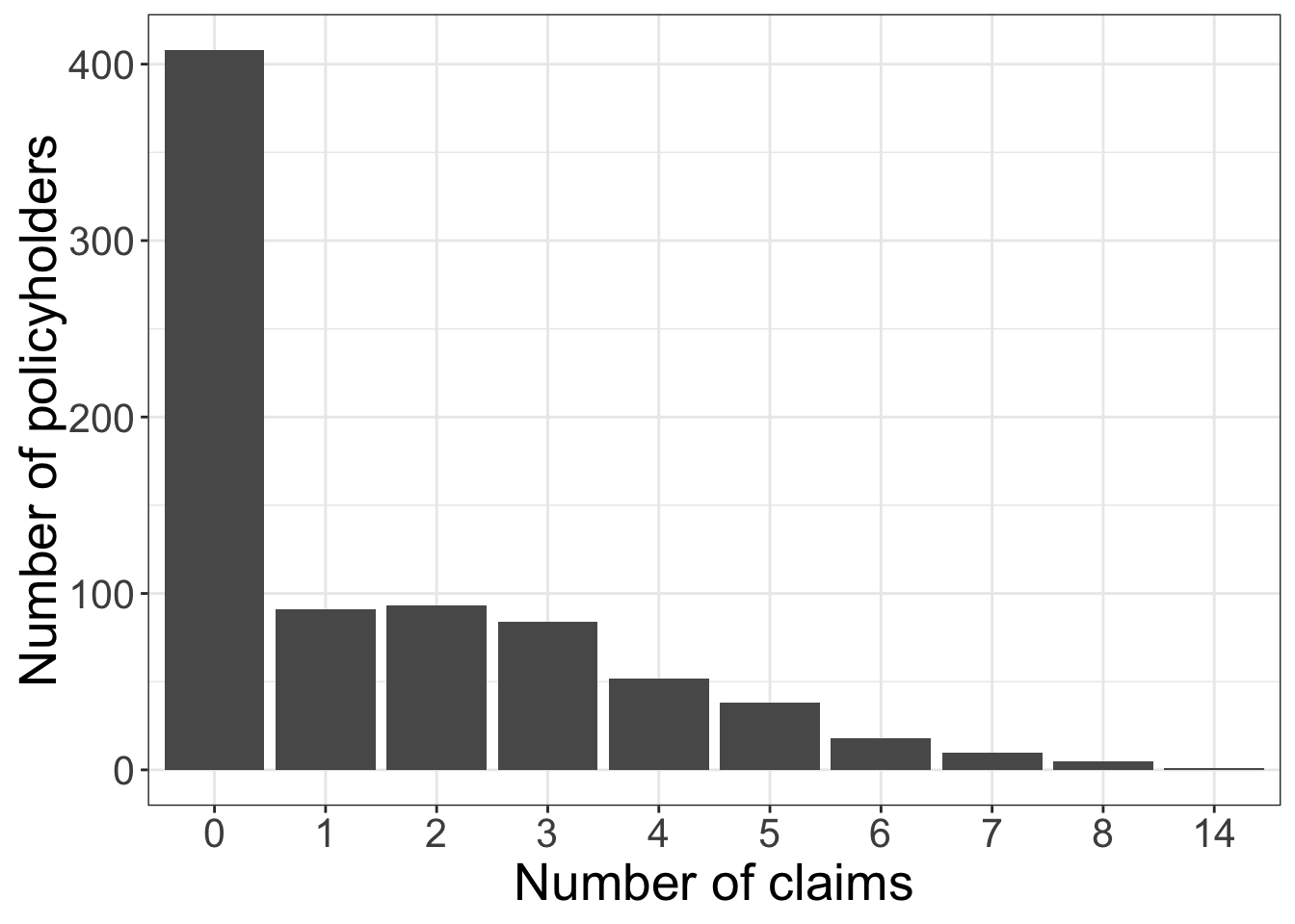
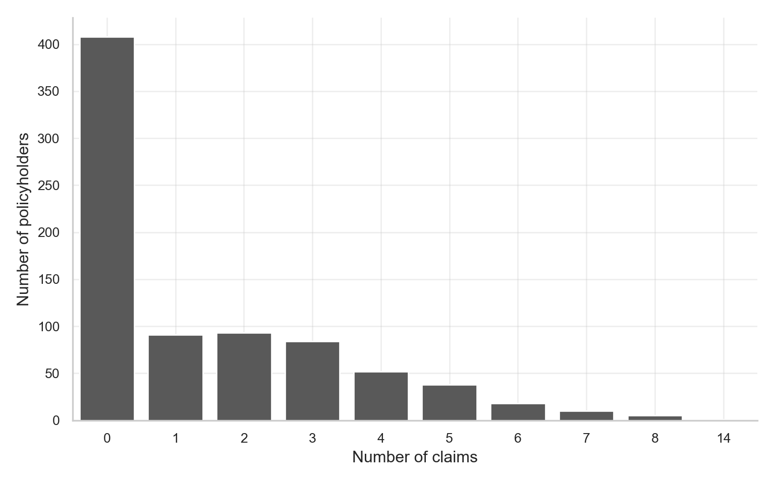
As shown in Figure 12.2 and Figure 12.3, the training-data distribution remains strongly concentrated at zero and then declines through the positive counts. In the training set, there are 408 zero-claim policyholders out of 800 training observations, while the maximum observed count is 14. This visual pattern is the first sign that a one-process Poisson model may not be flexible enough.
The next table compares the observed zero rate in the training data with the zero rate implied by a Poisson distribution whose mean equals the training-set sample mean.
claims_summary <- train_data |>
  summarise(
    `Number of observations` = n(),
    `Number of zeros` = sum(claims == 0, na.rm = TRUE),
    `Proportion of zeros` = mean(claims == 0, na.rm = TRUE),
    `Sample mean` = mean(claims, na.rm = TRUE),
    `Sample variance` = var(claims, na.rm = TRUE),
    `Variance-to-mean ratio` = var(claims, na.rm = TRUE) / mean(claims, na.rm = TRUE),
    `Poisson expected zero rate` = exp(-mean(claims, na.rm = TRUE)),
    `Excess zero rate` = mean(claims == 0, na.rm = TRUE) - exp(-mean(claims, na.rm = TRUE)),
    `Maximum` = max(claims, na.rm = TRUE)
  ) |>
  pivot_longer(
    cols = everything(),
    names_to = "Summary",
    values_to = "Value"
  )

claims_summary |>
  fmt_table() |>
    print_as_dt()
y_train_eda = training_data["claims"]
claims_summary = pd.Series({
"Number of observations": len(y_train_eda),
"Number of zeros": int((y_train_eda == 0).sum()),
"Proportion of zeros": (y_train_eda == 0).mean(),
"Sample mean": y_train_eda.mean(),
"Sample variance": y_train_eda.var(ddof=1),
"Variance-to-mean ratio": y_train_eda.var(ddof=1) / y_train_eda.mean(),
"Poisson expected zero rate": np.exp(-y_train_eda.mean()),
"Excess zero rate": (y_train_eda == 0).mean() - np.exp(-y_train_eda.mean()),
"Maximum": y_train_eda.max()
}).reset_index()
claims_summary.columns = ["Summary", "Value"]This table formalises the visual insight from Figure 12.2. In the training data, the sample mean is 1.449, the sample variance is 3.725, and the variance-to-mean ratio is 2.571. A Poisson distribution with the same mean would imply an expected zero rate of about 0.2349, but the observed zero rate is 0.51. The difference, 0.2751, is a simple empirical measure of excess zeros.
12.4.2 Zero claims versus nonzero claims
The next comparison keeps the count response intact, but splits the training data into observations with zero claims and observations with at least one claim. This table is especially useful because ZIP regression is motivated by the possibility that the zero and count-generating parts of the data behave differently.
zero_group_summary <- train_data |>
  group_by(has_claim) |>
  summarise(
    n = n(),
    mean_driver_age = mean(driver_age, na.rm = TRUE),
    mean_annual_mileage = mean(annual_mileage, na.rm = TRUE),
    mean_vehicle_age = mean(vehicle_age, na.rm = TRUE),
    male_rate = mean(male, na.rm = TRUE),
    urban_rate = mean(urban_area, na.rm = TRUE),
    prior_claims_rate = mean(prior_claims, na.rm = TRUE),
    mean_claims = mean(claims, na.rm = TRUE),
    .groups = "drop"
  ) |>
  mutate(
    claim_status = if_else(has_claim == 0, "Zero claims", "At least one claim")
  ) |>
  select(claim_status, everything(), -has_claim)

zero_group_summary_display <- zero_group_summary |>
  mutate(
    claim_status = factor(
      claim_status,
      levels = c("Zero claims", "At least one claim")
    )
  ) |>
  pivot_longer(
    cols = -claim_status,
    names_to = "Statistic",
    values_to = "Value"
  ) |>
  mutate(
    Statistic = recode(
      Statistic,
      n = "Number of observations",
      mean_driver_age = "Mean driver age",
      mean_annual_mileage = "Mean annual mileage",
      mean_vehicle_age = "Mean vehicle age",
      male_rate = "Male rate",
      urban_rate = "Urban-area rate",
      prior_claims_rate = "Prior-claims rate",
      mean_claims = "Mean claims"
    )
  ) |>
  pivot_wider(
    names_from = claim_status,
    values_from = Value
  )

zero_group_summary_display |>
  fmt_table() |>
    print_as_dt()
zero_group_summary = (
training_data.groupby("has_claim")
.agg(
n=("claims", "size"),
mean_driver_age=("driver_age", "mean"),
mean_annual_mileage=("annual_mileage", "mean"),
mean_vehicle_age=("vehicle_age", "mean"),
male_rate=("male", "mean"),
urban_rate=("urban_area", "mean"),
prior_claims_rate=("prior_claims", "mean"),
mean_claims=("claims", "mean")
)
.reset_index()
)
zero_group_summary["claim_status"] = zero_group_summary["has_claim"].map({
0: "Zero claims",
1: "At least one claim"
})
zero_group_summary = zero_group_summary.drop(columns="has_claim")
statistic_labels = {
"n": "Number of observations",
"mean_driver_age": "Mean driver age",
"mean_annual_mileage": "Mean annual mileage",
"mean_vehicle_age": "Mean vehicle age",
"male_rate": "Male rate",
"urban_rate": "Urban-area rate",
"prior_claims_rate": "Prior-claims rate",
"mean_claims": "Mean claims",
}
statistic_order = list(statistic_labels.values())
claim_status_order = ["Zero claims", "At least one claim"]
zero_group_summary_display = zero_group_summary.melt(
id_vars="claim_status",
var_name="Statistic",
value_name="Value"
)
zero_group_summary_display["Statistic"] = zero_group_summary_display["Statistic"].map(statistic_labels)
zero_group_summary_display["Statistic"] = pd.Categorical(
zero_group_summary_display["Statistic"],
categories=statistic_order,
ordered=True
)
zero_group_summary_display["claim_status"] = pd.Categorical(
zero_group_summary_display["claim_status"],
categories=claim_status_order,
ordered=True
)
zero_group_summary_display = (
zero_group_summary_display
.pivot(index="Statistic", columns="claim_status", values="Value")
.reset_index()
)
zero_group_summary_display.columns.name = None
zero_group_summary_display = zero_group_summary_display[
["Statistic", "Zero claims", "At least one claim"]
]The training-data EDA shows that the nonzero-claim group drives more miles on average: 17020 annual miles compared with 13570 for the zero-claim group. The prior-claims rate is also higher among policyholders with at least one claim during the study period: 0.3214 compared with 0.1225. This does not prove a causal mechanism, but it suggests that mileage and prior claims may help distinguish the zero and nonzero portions of the response.
12.4.3 Binary covariates
The binary covariates provide a compact way to inspect whether group membership is associated with different average counts and different zero rates in the training data.
binary_cols <- c("male", "urban_area", "prior_claims")

binary_summary <- purrr::map_dfr(binary_cols, function(col) {
  train_data |>
    group_by(value = .data[[col]]) |>
    summarise(
      n = n(),
      mean_claims = mean(claims, na.rm = TRUE),
      var_claims = var(claims, na.rm = TRUE),
      zero_rate = mean(claims == 0, na.rm = TRUE),
      nonzero_rate = mean(claims > 0, na.rm = TRUE),
      max_claims = max(claims, na.rm = TRUE),
      .groups = "drop"
    ) |>
    mutate(variable = col, .before = 1)
})

binary_summary |>
  fmt_table() |>
    print_as_dt()
binary_cols = ["male", "urban_area", "prior_claims"]
binary_summary = []
for col in binary_cols:
summary = (
training_data.groupby(col)
.agg(
n=("claims", "size"),
mean_claims=("claims", "mean"),
var_claims=("claims", "var"),
zero_rate=("claims", lambda x: (x == 0).mean()),
nonzero_rate=("claims", lambda x: (x > 0).mean()),
max_claims=("claims", "max")
)
.reset_index()
.rename(columns={col: "value"})
)
summary.insert(0, "variable", col)
binary_summary.append(summary)
binary_summary = pd.concat(binary_summary, ignore_index=True)The strongest binary-covariate contrast in the training-data EDA is expected to remain prior_claims. Policyholders with prior claims have a mean of about 2.477 claims and a zero rate of about 0.2841; those without prior claims have a mean of about 1.159 claims and a zero rate of about 0.5737. By contrast, the urban_area groups differ by about 0.1358 in mean claims and 0.04536 in zero rate in this training set.
12.4.4 Continuous covariates and visual trends
The continuous covariates can be inspected through scatterplots and binned summaries. Because the response is a discrete count, points stack horizontally at integer values.
continuous_data <- train_data |>
  select(claims, driver_age, annual_mileage, vehicle_age) |>
  pivot_longer(
    cols = c(driver_age, annual_mileage, vehicle_age),
    names_to = "covariate",
    values_to = "value"
  )

ggplot(continuous_data, aes(x = value, y = claims)) +
  geom_point(alpha = 0.35) +
  facet_wrap(~ covariate, scales = "free_x") +
  labs(
    x = "Covariate value",
    y = "Number of claims"
  ) +
  zip_theme
continuous_cols = ["driver_age", "annual_mileage", "vehicle_age"]
covariate_labels = {
"driver_age": "Driver age",
"annual_mileage": "Annual mileage",
"vehicle_age": "Vehicle age",
}
plt.close("all")
fig, axes = plt.subplots(
nrows=1,
ncols=len(continuous_cols),
figsize=(14, 4.5),
sharey=True
)
for ax, col in zip(axes, continuous_cols):
plot_data = training_data[[col, "claims"]].copy()
plot_data[col] = pd.to_numeric(plot_data[col], errors="coerce")
plot_data["claims"] = pd.to_numeric(plot_data["claims"], errors="coerce")
sns.scatterplot(
data=plot_data,
x=col,
y="claims",
color=ZIP_POINT_COLOR,
alpha=0.35,
edgecolor=None,
s=28,
ax=ax
)
ax.set_title(covariate_labels[col])
ax.set_xlabel("Covariate value")
ax.set_ylabel("Number of claims" if col == continuous_cols[0] else "")
zip_clean_axis(ax)
plt.tight_layout()
plt.show()
plt.close(fig)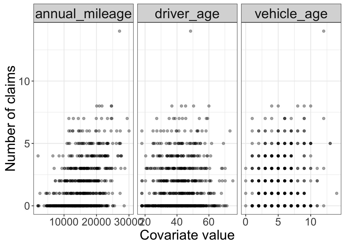
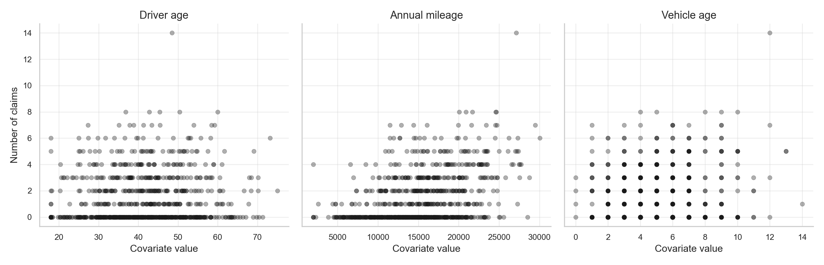
As shown in Figure 12.4 and Figure 12.5, annual mileage displays the clearest positive marginal pattern: higher-mileage policyholders are more likely to appear among the larger claim counts. Vehicle age shows a weaker positive pattern, while driver age has a more modest relationship.
Binned summaries make these patterns easier to read.
make_binned_summary <- function(df, variable, bins = 6) {
  x <- df[[variable]]
  bin_breaks <- seq(
    min(x, na.rm = TRUE),
    max(x, na.rm = TRUE),
    length.out = bins + 1
  )

  df |>
    mutate(
      variable = .env$variable,
      bin_id = cut(
        .data[[variable]],
        breaks = bin_breaks,
        include.lowest = TRUE,
        labels = FALSE
      ),
      bin = cut(
        .data[[variable]],
        breaks = bin_breaks,
        include.lowest = TRUE,
        dig.lab = 6
      ),
      bin_lower = bin_breaks[bin_id],
      bin_upper = bin_breaks[bin_id + 1],
      bin_midpoint = (bin_lower + bin_upper) / 2,
      bin_width = bin_upper - bin_lower
    ) |>
    filter(!is.na(bin_id)) |>
    group_by(
      variable,
      bin_id,
      bin,
      bin_lower,
      bin_upper,
      bin_midpoint,
      bin_width
    ) |>
    summarise(
      n = n(),
      mean_claims = mean(claims, na.rm = TRUE),
      zero_rate = mean(claims == 0, na.rm = TRUE),
      .groups = "drop"
    ) |>
    arrange(variable, bin_midpoint)
}

binned_summary <- bind_rows(
  make_binned_summary(train_data, "driver_age"),
  make_binned_summary(train_data, "annual_mileage"),
  make_binned_summary(train_data, "vehicle_age")
)

binned_summary |>
  select(variable, bin, bin_midpoint, n, mean_claims, zero_rate) |>
  mutate(bin = as.character(bin)) |>
  fmt_table() |>
    print_as_dt()
continuous_cols = ["driver_age", "annual_mileage", "vehicle_age"]
binned_summaries = []
def fmt_axis_value(x):
if abs(x) >= 1000:
return f"{x:,.0f}"
if abs(x - round(x)) < 1e-8:
return f"{x:.0f}"
return f"{x:.1f}"
def fmt_interval(left, right, first=False):
left_bracket = "[" if first else "("
return f"{left_bracket}{fmt_axis_value(left)}, {fmt_axis_value(right)}]"
for col in continuous_cols:
temp = training_data.copy()
temp[col] = pd.to_numeric(temp[col], errors="coerce")
temp["claims"] = pd.to_numeric(temp["claims"], errors="coerce")
bin_edges = np.linspace(temp[col].min(), temp[col].max(), 7)
temp["bin_id"] = (
pd.cut(
temp[col],
bins=bin_edges,
include_lowest=True,
labels=False
)
.astype("Int64") + 1
)
summary = (
temp.dropna(subset=["bin_id"])
.groupby("bin_id", observed=True)
.agg(
n=("claims", "size"),
mean_claims=("claims", "mean"),
zero_rate=("claims", lambda x: (x == 0).mean())
)
.reset_index()
)
summary.insert(0, "variable", col)
summary["bin_lower"] = summary["bin_id"].apply(lambda i: bin_edges[int(i) - 1])
summary["bin_upper"] = summary["bin_id"].apply(lambda i: bin_edges[int(i)])
summary["bin_midpoint"] = (summary["bin_lower"] + summary["bin_upper"]) / 2
summary["bin_width"] = summary["bin_upper"] - summary["bin_lower"]
summary["bin"] = summary.apply(
lambda row: fmt_interval(
row["bin_lower"],
row["bin_upper"],
first=int(row["bin_id"]) == 1
),
axis=1
)
binned_summaries.append(summary)
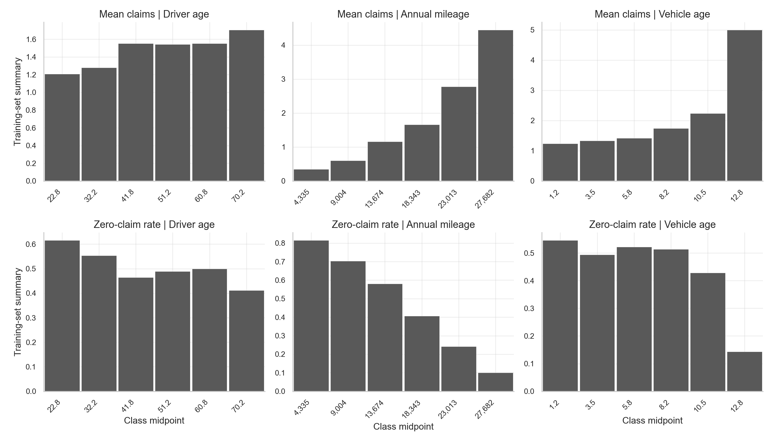
binned_summary = pd.concat(binned_summaries, ignore_index=True)The binned EDA indicates that annual mileage is the most pronounced continuous covariate. In the training data, the mean number of claims rises from about 0.3421 in the lowest mileage bin to about 4.45 in the highest mileage bin, while the zero-claim rate falls from about 0.8158 to about 0.1. This pattern supports including annual_mileage in both the count and zero-inflation components of the model.
The following plot visualizes the same binned summaries from Table 12.13, making it easier to compare the direction of the mean-count and zero-rate patterns across the continuous covariates.
binned_plot_data <- binned_summary |>
  mutate(
    variable = factor(
      variable,
      levels = c("driver_age", "annual_mileage", "vehicle_age"),
      labels = c("Driver age", "Annual mileage", "Vehicle age")
    )
  ) |>
  pivot_longer(
    cols = c(mean_claims, zero_rate),
    names_to = "metric",
    values_to = "value"
  ) |>
  mutate(
    metric = recode(
      metric,
      mean_claims = "Mean claims",
      zero_rate = "Zero-claim rate"
    ),
    metric = factor(metric, levels = c("Mean claims", "Zero-claim rate"))
  )

midpoint_breaks <- sort(unique(binned_plot_data$bin_midpoint))

ggplot(binned_plot_data) +
  geom_rect(
    aes(
      xmin = bin_lower,
      xmax = bin_upper,
      ymin = 0,
      ymax = value
    ),
    fill = "grey35",
    color = "white",
    linewidth = 0.25
  ) +
  facet_grid(metric ~ variable, scales = "free") +
  scale_x_continuous(
    breaks = function(lims) {
      midpoint_breaks[midpoint_breaks >= lims[1] & midpoint_breaks <= lims[2]]
    },
    labels = function(x) {
      format(signif(x, 4), big.mark = ",", scientific = FALSE, trim = TRUE)
    },
    expand = expansion(mult = c(0.01, 0.01))
  ) +
  labs(
    x = "Class midpoint",
    y = "Training-set summary"
  ) +
  theme_bw() +
  theme(
    axis.text = element_text(size = 10),
    axis.text.x = element_text(angle = 45, hjust = 1),
    axis.title.x = element_text(size = 14),
    axis.title.y = element_text(size = 14, vjust = 0.5),
    strip.text = element_text(size = 12),
    legend.position = "bottom",
    panel.spacing.x = unit(0.45, "lines"),
    panel.spacing.y = unit(0.45, "lines")
)plt.close("all")
binned_plot_data = binned_summary.copy()
variable_order = ["driver_age", "annual_mileage", "vehicle_age"]
variable_labels = {
"driver_age": "Driver age",
"annual_mileage": "Annual mileage",
"vehicle_age": "Vehicle age",
}
metric_order = ["Mean claims", "Zero-claim rate"]
binned_plot_data = binned_plot_data.melt(
id_vars=[
"variable",
"bin",
"bin_id",
"bin_lower",
"bin_upper",
"bin_midpoint",
"bin_width"
],
value_vars=["mean_claims", "zero_rate"],
var_name="metric",
value_name="value"
)
binned_plot_data["metric"] = binned_plot_data["metric"].map({
"mean_claims": "Mean claims",
"zero_rate": "Zero-claim rate"
})
fig, axes = plt.subplots(
nrows=len(metric_order),
ncols=len(variable_order),
figsize=ZIP_WIDE_FIGSIZE,
sharey=False
)
for row_idx, metric in enumerate(metric_order):
for col_idx, variable in enumerate(variable_order):
ax = axes[row_idx, col_idx]
plot_data = (
binned_plot_data[
(binned_plot_data["metric"] == metric)
& (binned_plot_data["variable"] == variable)
]
.sort_values("bin_midpoint")
.copy()
)
ax.bar(
x=plot_data["bin_midpoint"],
height=plot_data["value"],
width=plot_data["bin_width"] * 0.95,
align="center",
color=ZIP_BAR_COLOR,
edgecolor="white",
linewidth=0.25
)
ax.set_xticks(plot_data["bin_midpoint"])
ax.set_xticklabels(
[fmt_axis_value(x) for x in plot_data["bin_midpoint"]],
rotation=45,
ha="right"
)
ax.set_xlim(
plot_data["bin_lower"].min(),
plot_data["bin_upper"].max()
)
ax.set_title(f"{metric} | {variable_labels[variable]}")
ax.set_xlabel("Class midpoint" if row_idx == len(metric_order) - 1 else "")
ax.set_ylabel("Training-set summary" if col_idx == 0 else "")
zip_clean_axis(ax)
plt.subplots_adjust(wspace=0.22, hspace=0.55)
plt.tight_layout()
plt.show()
plt.close(fig)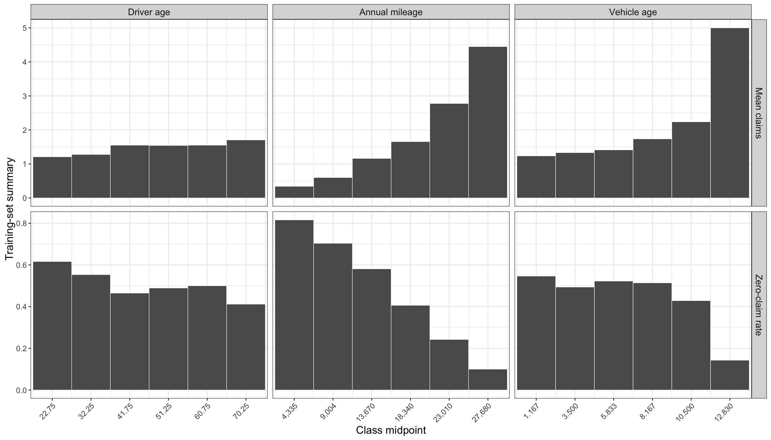
12.4.5 Correlation summary
The final EDA table gives a compact numerical summary of the marginal associations between each covariate, the original count response, and the binary has_claim indicator.
correlation_summary <- train_data |>
  select(driver_age, annual_mileage, vehicle_age, male, urban_area, prior_claims, claims, has_claim) |>
  summarise(across(
    c(driver_age, annual_mileage, vehicle_age, male, urban_area, prior_claims),
    list(
      corr_with_claims = ~ cor(.x, claims),
      corr_with_has_claim = ~ cor(.x, has_claim)
    ),
    .names = "{.col}_{.fn}"
  )) |>
  pivot_longer(
    cols = everything(),
    names_to = c("variable", ".value"),
    names_pattern = "(.*)_(corr_with_.*)"
  )

correlation_summary |>
  fmt_table() |>
    print_as_dt()
corr = training_data[[
"driver_age", "annual_mileage", "vehicle_age", "male",
"urban_area", "prior_claims", "claims", "has_claim"
]].corr()
correlation_summary = pd.DataFrame({
"corr_with_claims": corr["claims"].drop(["claims", "has_claim"]),
"corr_with_has_claim": corr["has_claim"].drop(["claims", "has_claim"])
}).reset_index(names="variable")The correlation summary reinforces the graphical EDA. In the training data, annual_mileage has the strongest correlation with claims, about 0.4062, and with has_claim, about 0.3384. prior_claims is also notable, with correlations of about 0.2832 with claims and 0.24 with has_claim. These correlations do not establish causality, but they help explain why these covariates are sensible choices for the model components.
One caution is worth keeping in mind before moving from EDA to modelling. These marginal summaries inspect each covariate mostly one at a time, but the fitted regression model will estimate the contribution of each regressor while holding the others fixed. If two covariates tend to move together, the apparent pattern for one variable may partly reflect the influence of another. For example, the plots and summaries suggest strong patterns for annual_mileage and prior_claims, but later coefficient interpretation should still be read as a model-based adjusted statement rather than as a direct copy of the marginal EDA pattern.
12.4.6 EDA summary
The exploratory analysis points to two connected conclusions. First, claims is a count response with a large concentration at zero. Second, the covariates do not all show the same marginal relationship with the response, so the later ZIP model should be allowed to separate the zero-generating mechanism from the count-generating mechanism.
| EDA Theme | TLDR | Dynamic Evidence | Modelling Implication |
|---|---|---|---|
| Response shape | The response is heavily concentrated at zero, with a smaller right tail of positive claim counts. | There are 408 zero-claim observations out of 800 training observations; the largest observed count is 14. | A count model is needed, but the zero pile-up should be modelled explicitly. |
| Mean - variance pattern | The response is more variable than a simple equidispersed Poisson pattern would suggest. | The sample mean is 1.449, the sample variance is 3.725, and the variance-to-mean ratio is 2.571. | A one-process Classical Poisson model may be too restrictive. |
| Zero inflation check | The observed zero rate is larger than the zero rate implied by a Poisson model with the same mean. | The observed zero rate is 0.51, while the Poisson-expected zero rate is 0.2349; the excess zero rate is 0.2751. | This is direct empirical motivation for a zero-inflated model. |
| Zero versus nonzero profiles | Policyholders with at least one claim tend to have higher mileage and a higher prior-claims rate. | Mean annual mileage is 17020 for nonzero-claim policyholders versus 13570 for zero-claim policyholders; the prior-claims rate is 0.3214 versus 0.1225. |
annual_mileage and prior_claims are plausible regressors for both claim frequency and the zero/nonzero distinction. |
| Binary covariates |
prior_claims shows the clearest binary-covariate contrast; urban_area is weaker in this training split. |
With prior claims, mean claims are 2.477 and the zero rate is 0.2841; without prior claims, mean claims are 1.159 and the zero rate is 0.5737. The urban groups differ by about 0.1358 in mean claims and 0.04536 in zero rate. |
prior_claims should be treated as an important candidate covariate; urban_area may still be retained for substantive insurance interpretation. |
| Continuous covariates |
annual_mileage has the clearest positive marginal association with the response. |
Mean claims rise from 0.3421 in the lowest mileage bin to 4.45 in the highest mileage bin; the zero rate falls from 0.8158 to 0.1. Its correlations are 0.4062 with claims and 0.3384 with has_claim. |
annual_mileage is a natural candidate for the count component and the zero-inflation component. |
| Covariate interpretation caution | Marginal EDA patterns are useful, but they do not isolate each regressor’s adjusted contribution. |
annual_mileage and prior_claims both show strong relationships with claims and has_claim, so their fitted coefficients should later be interpreted conditionally on the other model terms. |
Later model interpretation should distinguish descriptive marginal patterns from adjusted regression effects. |
12.5 Preparing for Modelling
The data schema confirms that the response is a zero-inflated count and that the available regressors are either continuous, integer-valued, or binary. There are no multi-category nominal covariates in this dataset, so we do not need to create a baseline category plus a collection of dummy variables. The binary covariates are already coded as \(0/1\) indicators, and the continuous or integer-valued regressors can enter the model directly unless a later modelling choice calls for centering, scaling, or nonlinear transformations.
For policyholder \(i\), define the response as
\[Y_i = \texttt{claims}_i,\]
where \(Y_i\) is the number of claims filed during the observation window. The candidate covariates are indexed in the same order as the variable table above, excluding the response.
| Symbol | Coding Name Alias | Variable Meaning | Type | Binary Coding |
|---|---|---|---|---|
| \(x_{1,i}\) | driver_age |
Age of policyholder \(i\), measured in years. | Continuous | Not binary. |
| \(x_{2,i}\) | annual_mileage |
Total kilometers driven per year by policyholder \(i\). | Continuous | Not binary. |
| \(x_{3,i}\) | vehicle_age |
Age of the insured vehicle for policyholder \(i\), measured in years. | Discrete | Not binary; integer-valued from 0 to 20. |
| \(x_{4,i}\) | male |
Sex indicator for policyholder \(i\). | Discrete | \(1\) means male; \(0\) means female. |
| \(x_{5,i}\) | urban_area |
Primary driving-environment indicator for policyholder \(i\). | Discrete | \(1\) means urban; \(0\) means rural. |
| \(x_{6,i}\) | prior_claims |
Prior-claims-history indicator for policyholder \(i\). | Discrete | \(1\) means the driver filed claims in previous years; \(0\) means no prior claims. |
Using this notation, a compact covariate vector for the full set of candidate regressors is
\[\mathbf{x}_i = \left(1, x_{1,i}, x_{2,i}, x_{3,i}, x_{4,i}, x_{5,i}, x_{6,i}\right)\]
Where the leading \(1\) represents the intercept. In the ZIP model, this covariate vector can be used to build two linked regression components: a count component for the expected number of claims among policyholders in the count-generating process, and a zero-inflation component for the probability of belonging to the extra-zero group. Later sections can choose whether both components use the same covariates or whether one component uses a smaller, substantively motivated subset.
12.6 Comparing to Other Approaches
Before introducing the full Zero-Inflated Poisson (ZIP) model, it is useful to compare it with two simpler approaches that each captures only part of the modelling problem. The goal of this comparison is not only to fit two baselines, but also to see what each baseline reveals about the insurance-claims data.
First, we can turn the count response into a binary response. Define \(H_i = \mathbb{I}(Y_i > 0)\) where \(Y_i\) is the number of claims for policyholder \(i\), and \(\mathbb{I}\) is the indicator function, which outputs \(1\) in the case that \(Y_i>1\), and \(0\) in any other case. A Binary Logistic Regression model for has_claim then describes whether a policyholder filed at least one claim. This is directly connected to the large zero-versus-nonzero split observed in Figure 12.2 and Table 12.7, but it does not distinguish between one claim and several claims.
Second, we can keep the original count response and fit a Classical Poisson Regression model for claims. This model describes the expected number of claims directly, so it keeps the count scale used in Figure 12.4 and Table 12.13. However, it treats all observations as coming from a single count-generating process. In particular, it ties the zero rate to the same mean parameter that governs the positive counts.
These two models are not replacements for ZIP regression in this chapter. Instead, they give us useful comparison points. Logistic Regression focuses on the zero-versus-nonzero distinction. Classical Poisson Regression focuses on the count scale. ZIP regression combines these ideas by allowing a separate zero-generating component and a count-generating component.
12.6.1 Binary Logistic Regression for has_claim
Model definition
The Logistic Regression alternative uses the derived binary response in Equation 12.1.
\[H_i = \begin{cases} 1, & \text{if policyholder } i \text{ filed at least one claim}, \\ 0, & \text{if policyholder } i \text{ filed no claims}. \end{cases} \tag{12.1}\]
The probabilistic assumption is given in Equation 12.2, where \(\pi_i = P(H_i = 1 \mid \mathbf{x}_i)\) is the probability that policyholder \(i\) filed at least one claim.
\[H_i \mid \mathbf{x}_i \sim \operatorname{Bernoulli}(\pi_i) \tag{12.2}\]
The link function is the logit link in Equation 12.3.
\[\operatorname{logit}(\pi_i) = \log\left(\frac{\pi_i}{1 - \pi_i}\right) \tag{12.3}\]
Using the six covariates from the running example, the systematic component is shown in Equation 12.4.
\[\log\left(\frac{\pi_i}{1 - \pi_i}\right) = \alpha_0 + \alpha_1 x_{1,i} + \alpha_2 x_{2,i} + \alpha_3 x_{3,i} + \alpha_4 x_{4,i} + \alpha_5 x_{5,i} + \alpha_6 x_{6,i} \tag{12.4}\]
In Equation 12.4, there are \(7\) coefficients, \(\alpha_0, \alpha_1, \ldots, \alpha_6\), which change the log-odds of having at least one claim. The intercept \(\alpha_0\) is the baseline log-odds when all covariates are equal to zero, while \(\alpha_j\) for \(j \in \{1, 2, \ldots, 6\}\) represents the change in log-odds for a one-unit increase in the corresponding regressor \(x_{j,i}\), holding the other covariates fixed.
As in Chapter 8, this “one-unit increase” interpretation should be read according to the type of covariate. For a continuous covariate, such as driver_age or annual_mileage, \(\alpha_j\) describes the change in log-odds associated with increasing that covariate by one unit, holding the others fixed. For an integer-valued covariate, such as vehicle_age, the interpretation is similar, but the one-unit change corresponds to one additional year of vehicle age. For a binary indicator, such as male, urban_area, or prior_claims, \(\alpha_j\) compares the group coded \(1\) with the reference group coded \(0\). If a nominal categorical covariate with more than two categories were included, its coefficients would be interpreted relative to the omitted reference category, rather than as a literal one-unit increase.
In this formulation, the model describes the probability of at least one claim. It intentionally ignores the difference between one claim and multiple claims.
Heads-up on the connection to Chapter 8!
The logit link, Bernoulli assumption, and odds-ratio interpretation are introduced in Chapter 8. Here we use them only as a comparison point for the ZIP model, not as a full reintroduction of Binary Logistic Regression.
Fitting the model
For this comparison, we fit the model using the canonical training data created earlier in the chapter. The binary response has_claim is created explicitly in both languages so that the transformation from claims to \(H_i\) is visible.
train_data <- train_data |>
  mutate(has_claim = as.integer(claims > 0))

lr_model_r <- glm(
  has_claim ~ driver_age + annual_mileage + vehicle_age + male + urban_area + prior_claims,
  data = train_data,
  family = binomial(link = "logit")
)

broom::tidy(lr_model_r)
training_data = training_data.copy()
training_data["has_claim"] = (training_data["claims"] > 0).astype(int)
covariates = [
"driver_age",
"annual_mileage",
"vehicle_age",
"male",
"urban_area",
"prior_claims",
]
X = sm.add_constant(training_data[covariates], has_constant="add")
H = training_data["has_claim"]
lr_model_py = sm.Logit(H, X).fit(disp=False)
lr_coef_py = pd.DataFrame({
"term": lr_model_py.params.index,
"estimate": lr_model_py.params.values,
"std.error": lr_model_py.bse.values,
"statistic": lr_model_py.tvalues.values,
"p.value": lr_model_py.pvalues.values,
})Heads-up on R and Python model summaries!
The two outputs may not be formatted identically. R and Python use different summary conventions, and their numerical optimizers can differ in small implementation details. Because both chunks use the same canonical training split, the fitted coefficients should nevertheless be within similar ranges.
The coefficient table in Table 12.19 already points to the main event-probability story. The strongest positive fitted associations with has_claim are attached to annual_mileage and prior_claims, matching the EDA pattern in which higher-mileage policyholders and policyholders with prior claims were less concentrated at zero. driver_age is also positive in this binary model, but the fitted evidence is weaker than for mileage and prior claims. By contrast, vehicle_age, male, and urban_area are much flatter on the zero-versus-nonzero scale in this fit.
Interpreting the coefficients
The raw Logistic Regression coefficients are on the log-odds scale. To make them easier to read, the next table exponentiates scaled coefficient changes. The continuous covariates are rescaled to more meaningful comparisons: 10 years for driver_age, 10,000 km for annual_mileage, and 5 years for vehicle_age. Binary covariates are interpreted as the change from \(0\) to \(1\).
zip_interpret_scales <- tibble(
  term = c("driver_age", "annual_mileage", "vehicle_age", "male", "urban_area", "prior_claims"),
  comparison = c(
    "+10 years of driver age",
    "+10,000 km of annual mileage",
    "+5 years of vehicle age",
    "male (1) versus female (0)",
    "urban (1) versus rural (0)",
    "prior claims (1) versus none (0)"
  ),
  change = c(10, 10000, 5, 1, 1, 1)
)

coef_tbl <- broom::tidy(lr_model_r)
ci_tbl <- confint.default(lr_model_r) |>
  as.data.frame() |>
  tibble::rownames_to_column("term") |>
  rename(conf.low = `2.5 %`, conf.high = `97.5 %`)

lr_effects_r <- coef_tbl |>
  left_join(ci_tbl, by = "term") |>
  inner_join(zip_interpret_scales, by = "term") |>
  transmute(
    covariate = term,
    comparison,
    log_scale_change = estimate * change,
    odds_ratio = exp(estimate * change),
    lower_95 = exp(conf.low * change),
    upper_95 = exp(conf.high * change),
    percent_change = 100 * (exp(estimate * change) - 1),
    p_value = p.value
  )
scale_rows = pd.DataFrame({
"term": covariates,
"comparison": [
"+10 years of driver age",
"+10,000 km of annual mileage",
"+5 years of vehicle age",
"male (1) versus female (0)",
"urban (1) versus rural (0)",
"prior claims (1) versus none (0)",
],
"change": [10, 10000, 5, 1, 1, 1],
})
ci = lr_model_py.conf_int()
ci.columns = ["conf.low", "conf.high"]
coef = pd.DataFrame({
"term": lr_model_py.params.index,
"estimate": lr_model_py.params.values,
"conf.low": ci["conf.low"].values,
"conf.high": ci["conf.high"].values,
"p_value": lr_model_py.pvalues.values,
})
lr_effects_py = coef.merge(scale_rows, on="term", how="inner")
lr_effects_py["log_scale_change"] = lr_effects_py["estimate"] * lr_effects_py["change"]
lr_effects_py["odds_ratio"] = np.exp(lr_effects_py["log_scale_change"])
lr_effects_py["lower_95"] = np.exp(lr_effects_py["conf.low"] * lr_effects_py["change"])
lr_effects_py["upper_95"] = np.exp(lr_effects_py["conf.high"] * lr_effects_py["change"])
lr_effects_py["percent_change"] = 100 * (lr_effects_py["odds_ratio"] - 1)An odds ratio greater than \(1\) indicates higher odds of at least one claim for the stated comparison, holding the other covariates fixed. An odds ratio below \(1\) indicates lower odds. These are odds-scale statements, not direct probability differences.
The scaled effects in Table 12.21 make the size of the binary-response patterns clearer. Holding the other covariates fixed, a +10,000 km comparison in annual_mileage multiplies the fitted odds of at least one claim by about 5.448, while moving from no prior claims to prior claims multiplies the fitted odds by about 4.672. The +10 year driver_age comparison is positive but smaller, with an odds ratio of about 1.183. The remaining comparisons are much closer to the neutral value of \(1\) in this Logistic Regression model.
Visualizing the fitted Logistic Regression patterns
The next figures overlay empirical training-set summaries with fitted probabilities from the Logistic Regression model. For continuous covariates, the empirical points are binned averages. For binary covariates, the empirical points are group averages. The fitted curves or fitted line segments vary one covariate at a time while holding the remaining covariates at typical training-set values.
# Fitted probabilities were computed by varying one covariate at a time
# while holding the remaining covariates at typical training-set values.

ggplot() +
  geom_point(
    data = lr_observed_r,
    aes(x = x, y = observed),
    alpha = 0.85,
    size = 2
  ) +
  geom_line(
    data = lr_fitted_r,
    aes(x = x, y = fitted),
    linewidth = 1.1
  ) +
  facet_wrap(~ covariate_label, scales = "free_x") +
  scale_y_continuous(labels = scales::percent_format(accuracy = 1), limits = c(0, 1)) +
  labs(
    x = "Covariate value",
    y = "Probability of at least one claim"
  ) +
  zip_theme
# Fitted probabilities are computed by varying one covariate at a time
# while holding the remaining covariates at typical training-set values.
continuous_covariates = ["driver_age", "annual_mileage", "vehicle_age"]
binary_covariates = ["male", "urban_area", "prior_claims"]
labels = {
"driver_age": "Driver age",
"annual_mileage": "Annual mileage",
"vehicle_age": "Vehicle age",
"male": "Male indicator",
"urban_area": "Urban-area indicator",
"prior_claims": "Prior-claims indicator",
}
reference = {
"driver_age": training_data["driver_age"].median(),
"annual_mileage": training_data["annual_mileage"].median(),
"vehicle_age": training_data["vehicle_age"].median(),
"male": int(training_data["male"].mode().iloc[0]),
"urban_area": int(training_data["urban_area"].mode().iloc[0]),
"prior_claims": int(training_data["prior_claims"].mode().iloc[0]),
}
fig, axes = plt.subplots(2, 3, figsize=ZIP_WIDE_FIGSIZE, sharey=True)
axes = axes.flatten()
for ax, covariate in zip(axes, continuous_covariates + binary_covariates):
if covariate in binary_covariates:
grid_values = np.array([0, 1])
observed = (
training_data.groupby(covariate)["has_claim"]
.mean()
.reset_index()
.rename(columns={covariate: "x", "has_claim": "observed"})
)
else:
grid_values = np.linspace(training_data[covariate].min(), training_data[covariate].max(), 100)
temp = training_data[[covariate, "has_claim"]].copy()
temp["bin"] = pd.cut(temp[covariate], bins=6, include_lowest=True)
observed = (
temp.groupby("bin", observed=True)
.agg(x=(covariate, "mean"), observed=("has_claim", "mean"))
.reset_index(drop=True)
)
grid = pd.DataFrame([reference] * len(grid_values))
grid[covariate] = grid_values
X_grid = sm.add_constant(grid[zip_model_covariates_py], has_constant="add")
fitted = lr_model_py.predict(X_grid)
ax.scatter(observed["x"], observed["observed"], alpha=0.85, s=35)
ax.plot(grid_values, fitted, linewidth=1.8)
ax.set_title(labels[covariate])
ax.set_xlabel("Covariate value")
ax.set_ylabel("Probability of at least one claim")
ax.set_ylim(0, 1)
zip_clean_axis(ax)
plt.tight_layout()
plt.show()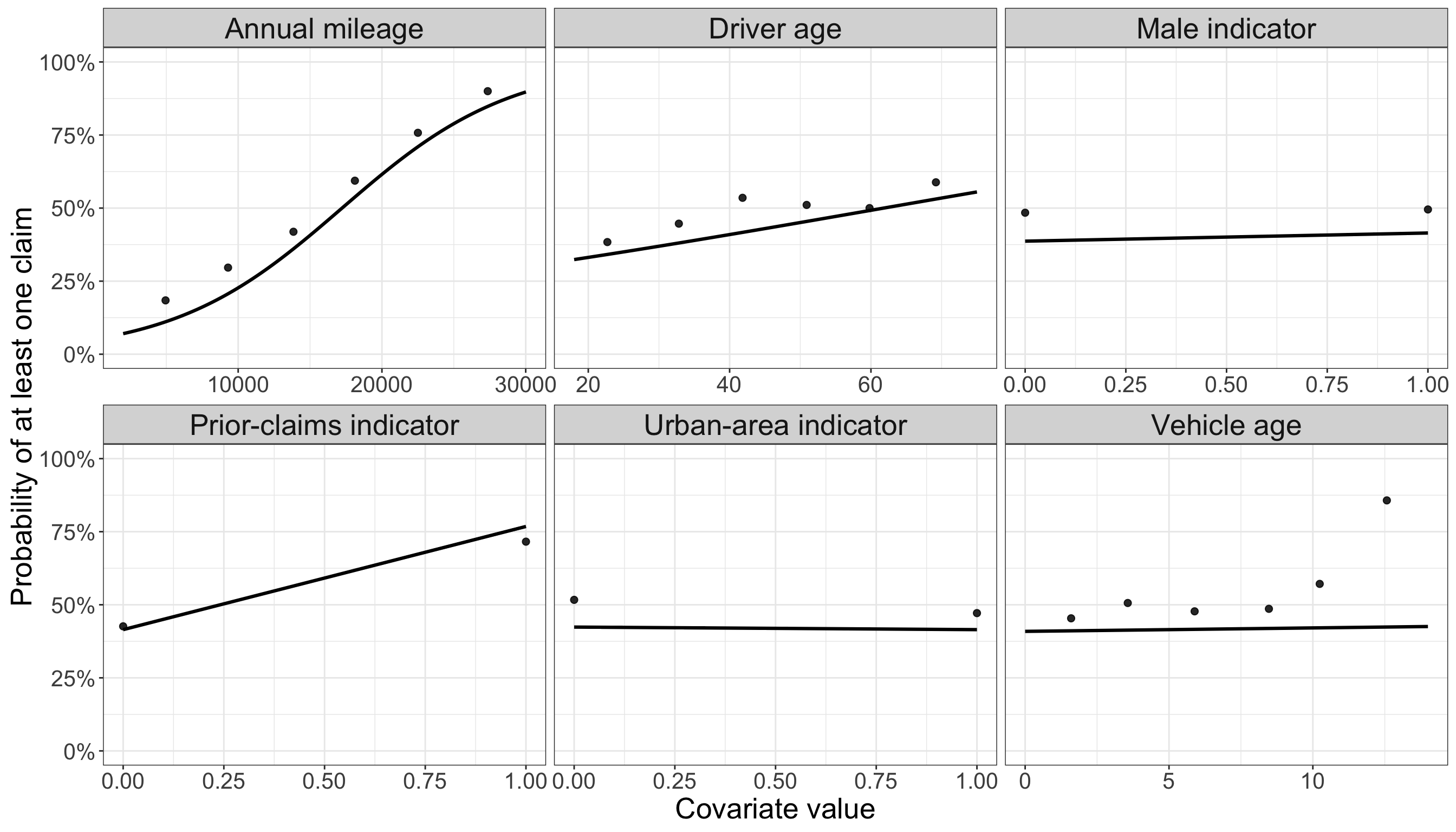
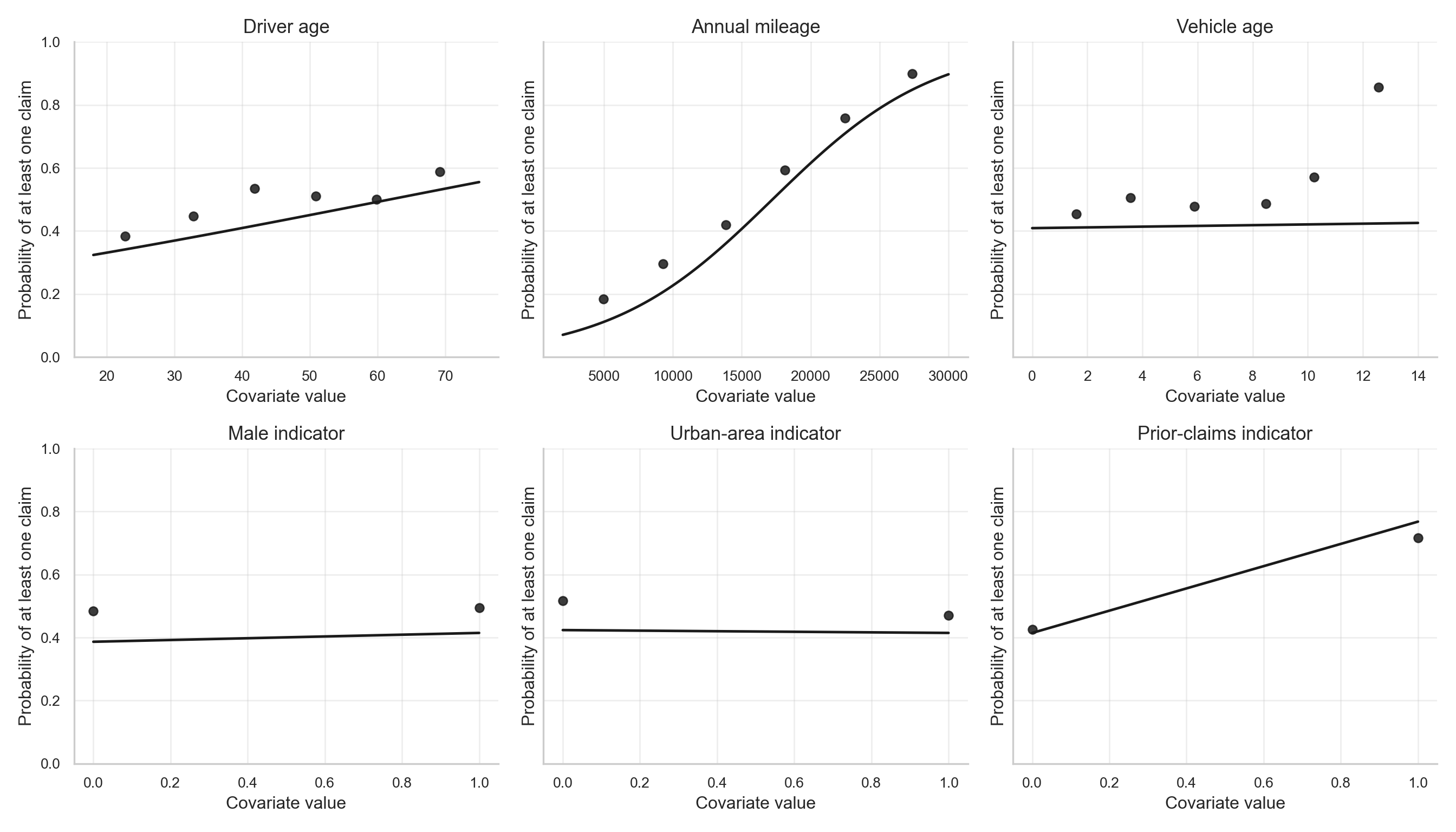
The fitted patterns in Figure 12.8 show the same message visually. When other covariates are held at typical training-set values, the fitted probability of at least one claim rises from about 7.035% at the low end of the mileage range to about 89.74% at the high end. The fitted prior-claims contrast is also visible: the fitted probability changes from about 41.49% for policyholders without prior claims to about 76.81% for policyholders with prior claims. The other panels are comparatively flatter, which is consistent with the smaller odds-ratio contrasts in Table 12.21.
This is exactly what Logistic Regression is meant to do: describe the probability that a policyholder enters the nonzero group. Its limitation is also visible from the original response distribution. Among training observations with at least one claim, the average positive count is 2.957, the maximum positive count is 14, and about 76.79% of nonzero-claim policyholders have more than one claim. After converting claims to has_claim, all of that frequency information is collapsed into \(H_i = 1\).
12.6.2 Classical Poisson Regression for claims
Model definition
The Classical Poisson Regression alternative keeps the original count response, defined in Equation 12.5.
\[Y_i = \text{number of claims filed by policyholder } i \tag{12.5}\]
The probabilistic assumption is shown in Equation 12.6, where \(\lambda_i = \mathbb{E}(Y_i \mid \mathbf{x}_i)\) is the expected number of claims for policyholder \(i\).
\[Y_i \mid \mathbf{x}_i \sim \operatorname{Poisson}(\lambda_i) \tag{12.6}\]
The link function is the log link in Equation 12.7.
\[g(\lambda_i) = \log(\lambda_i) \tag{12.7}\]
Using the same six covariates, the systematic component is given in Equation 12.8.
\[\log(\lambda_i) = \beta_0 + \beta_1 x_{1,i} + \beta_2 x_{2,i} + \beta_3 x_{3,i} + \beta_4 x_{4,i} + \beta_5 x_{5,i} + \beta_6 x_{6,i} \tag{12.8}\]
In Equation 12.8, there are \(7\) coefficients, \(\beta_0, \beta_1, \ldots, \beta_6\), which change the log-mean number of claims. The intercept \(\beta_0\) is the baseline log-mean when all covariates are equal to zero, while \(\beta_j\) for \(j \in \{1, 2, \ldots, 6\}\) represents the change in log-mean claims for a one-unit increase in the corresponding regressor \(x_{j,i}\), holding the other covariates fixed.
As in Chapter 10, this coefficient interpretation also depends on how the regressor is coded. For a continuous covariate, such as driver_age or annual_mileage, \(\beta_j\) describes the change in the log expected count for a one-unit increase in that covariate, holding the others fixed. For an integer-valued covariate, such as vehicle_age, the one-unit comparison corresponds to one additional year of vehicle age. For binary indicators, such as male, urban_area, or prior_claims, \(\beta_j\) compares the expected count for the group coded \(1\) against the reference group coded \(0\). If a nominal categorical covariate with more than two categories were included, its coefficients would compare each included category with the omitted reference category.
This model works directly on the count scale through \(\lambda_i\), but it also imposes the Poisson mean-variance relationship in Equation 12.9.
\[\mathbb{E}(Y_i \mid \mathbf{x}_i) = \operatorname{Var}(Y_i \mid \mathbf{x}_i) = \lambda_i \tag{12.9}\]
Heads-up on the connection to Chapter 10!
The Poisson probability model, log link, and rate-ratio interpretation are introduced in Chapter 10. Here we use Classical Poisson Regression as a baseline count model before moving to ZIP regression.
Fitting the model
X = sm.add_constant(training_data[covariates], has_constant="add")
Y = training_data["claims"]

cpr_model_py = sm.GLM(
    Y,
    X,
    family=sm.families.Poisson()
).fit()

cpr_coef_py = pd.DataFrame({
    "term": cpr_model_py.params.index,
    "estimate": cpr_model_py.params.values,
    "std.error": cpr_model_py.bse.values,
    "statistic": cpr_model_py.tvalues.values,
    "p.value": cpr_model_py.pvalues.values,
})Heads-up on R and Python model summaries!
As with the Logistic Regression output, the two outputs may not be formatted identically. R and Python use different summary conventions, and their numerical optimizers can differ in small implementation details. Because both chunks use the same canonical training split, the fitted coefficients should nevertheless be within similar ranges.
The coefficient table in Table 12.23 tells a count-scale story rather than a zero-versus-nonzero story. annual_mileage and prior_claims remain strong positive predictors, but vehicle_age and male now also show clearer positive fitted associations with the expected number of claims. This is an important difference from the Logistic Regression fit: a covariate may be weak for predicting whether any claim occurs, but still matter for the expected number of claims once the count scale is preserved.
Interpreting the coefficients
Poisson Regression coefficients are on the log-mean scale. Exponentiating a coefficient gives a multiplicative effect on the expected count. The next table uses the same scaling choices as above so that the coefficient interpretation is easier to compare across the two approaches.
coef_tbl <- broom::tidy(cpr_model_r)
ci_tbl <- confint.default(cpr_model_r) |>
  as.data.frame() |>
  tibble::rownames_to_column("term") |>
  rename(conf.low = `2.5 %`, conf.high = `97.5 %`)

cpr_effects_r <- coef_tbl |>
  left_join(ci_tbl, by = "term") |>
  inner_join(zip_interpret_scales, by = "term") |>
  transmute(
    covariate = term,
    comparison,
    log_scale_change = estimate * change,
    rate_ratio = exp(estimate * change),
    lower_95 = exp(conf.low * change),
    upper_95 = exp(conf.high * change),
    percent_change = 100 * (exp(estimate * change) - 1),
    p_value = p.value
  )
ci = cpr_model_py.conf_int()
ci.columns = ["conf.low", "conf.high"]
coef = pd.DataFrame({
"term": cpr_model_py.params.index,
"estimate": cpr_model_py.params.values,
"conf.low": ci["conf.low"].values,
"conf.high": ci["conf.high"].values,
"p_value": cpr_model_py.pvalues.values,
})
cpr_effects_py = coef.merge(scale_rows, on="term", how="inner")
cpr_effects_py["log_scale_change"] = cpr_effects_py["estimate"] * cpr_effects_py["change"]
cpr_effects_py["rate_ratio"] = np.exp(cpr_effects_py["log_scale_change"])
cpr_effects_py["lower_95"] = np.exp(cpr_effects_py["conf.low"] * cpr_effects_py["change"])
cpr_effects_py["upper_95"] = np.exp(cpr_effects_py["conf.high"] * cpr_effects_py["change"])
cpr_effects_py["percent_change"] = 100 * (cpr_effects_py["rate_ratio"] - 1)A rate ratio greater than \(1\) means that the expected number of claims is higher for the stated comparison, holding the other covariates fixed. A rate ratio below \(1\) means that the expected number of claims is lower.
The scaled rate ratios in Table 12.25 show that the largest count-scale comparison is again annual_mileage: a +10,000 km comparison multiplies the fitted expected number of claims by about 2.889. The fitted rate ratio for prior_claims is about 2.237, and the +5 year vehicle_age comparison has a fitted rate ratio of about 1.306. These CPR effects are not identical to the Logistic Regression effects because they answer a different question: how the expected count changes, not only whether the count is positive.
Visualizing the fitted Poisson Regression patterns
The next figures overlay empirical mean claims with fitted Poisson means. As before, continuous covariates use binned empirical summaries, binary covariates use group summaries, and the fitted curves vary one covariate at a time while holding the remaining covariates fixed at typical training-set values.
ggplot() +
  geom_point(
    data = cpr_observed_r,
    aes(x = x, y = observed),
    alpha = 0.85,
    size = 2
  ) +
  geom_line(
    data = cpr_fitted_r,
    aes(x = x, y = fitted),
    linewidth = 1.1
  ) +
  facet_wrap(~ covariate_label, scales = "free_x") +
  labs(
    x = "Covariate value",
    y = "Mean number of claims"
  ) +
  zip_theme
fig, axes = plt.subplots(2, 3, figsize=ZIP_WIDE_FIGSIZE, sharey=False)
axes = axes.flatten()
for ax, covariate in zip(axes, continuous_covariates + binary_covariates):
if covariate in binary_covariates:
grid_values = np.array([0, 1])
observed = (
training_data.groupby(covariate)["claims"]
.mean()
.reset_index()
.rename(columns={covariate: "x", "claims": "observed"})
)
else:
grid_values = np.linspace(training_data[covariate].min(), training_data[covariate].max(), 100)
temp = training_data[[covariate, "claims"]].copy()
temp["bin"] = pd.cut(temp[covariate], bins=6, include_lowest=True)
observed = (
temp.groupby("bin", observed=True)
.agg(x=(covariate, "mean"), observed=("claims", "mean"))
.reset_index(drop=True)
)
grid = pd.DataFrame([reference] * len(grid_values))
grid[covariate] = grid_values
X_grid = sm.add_constant(grid[zip_model_covariates_py], has_constant="add")
fitted = cpr_model_py.predict(X_grid)
ax.scatter(observed["x"], observed["observed"], alpha=0.85, s=35)
ax.plot(grid_values, fitted, linewidth=1.8)
ax.set_title(labels[covariate])
ax.set_xlabel("Covariate value")
ax.set_ylabel("Mean number of claims")
zip_clean_axis(ax)
plt.tight_layout()
plt.show()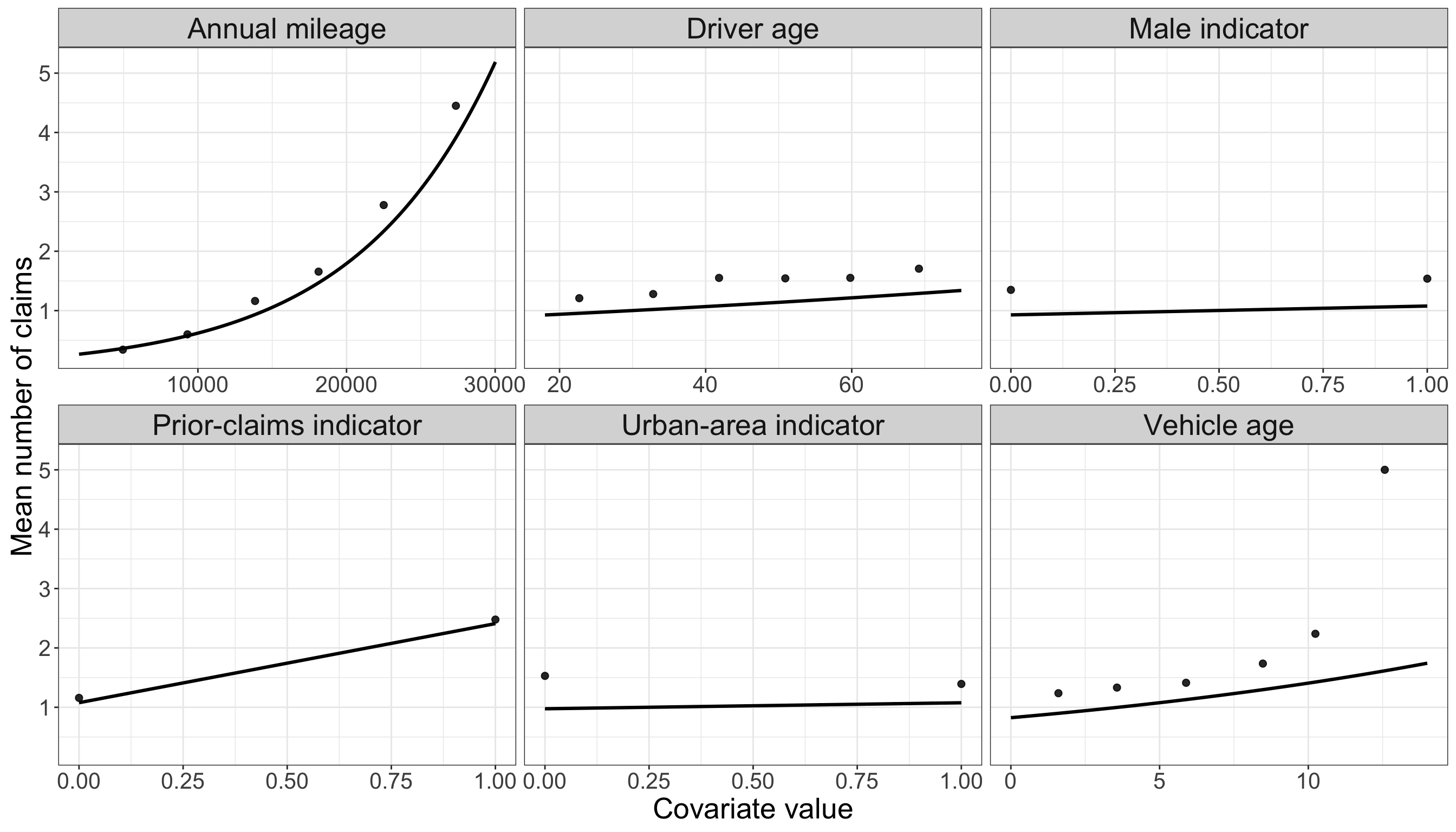
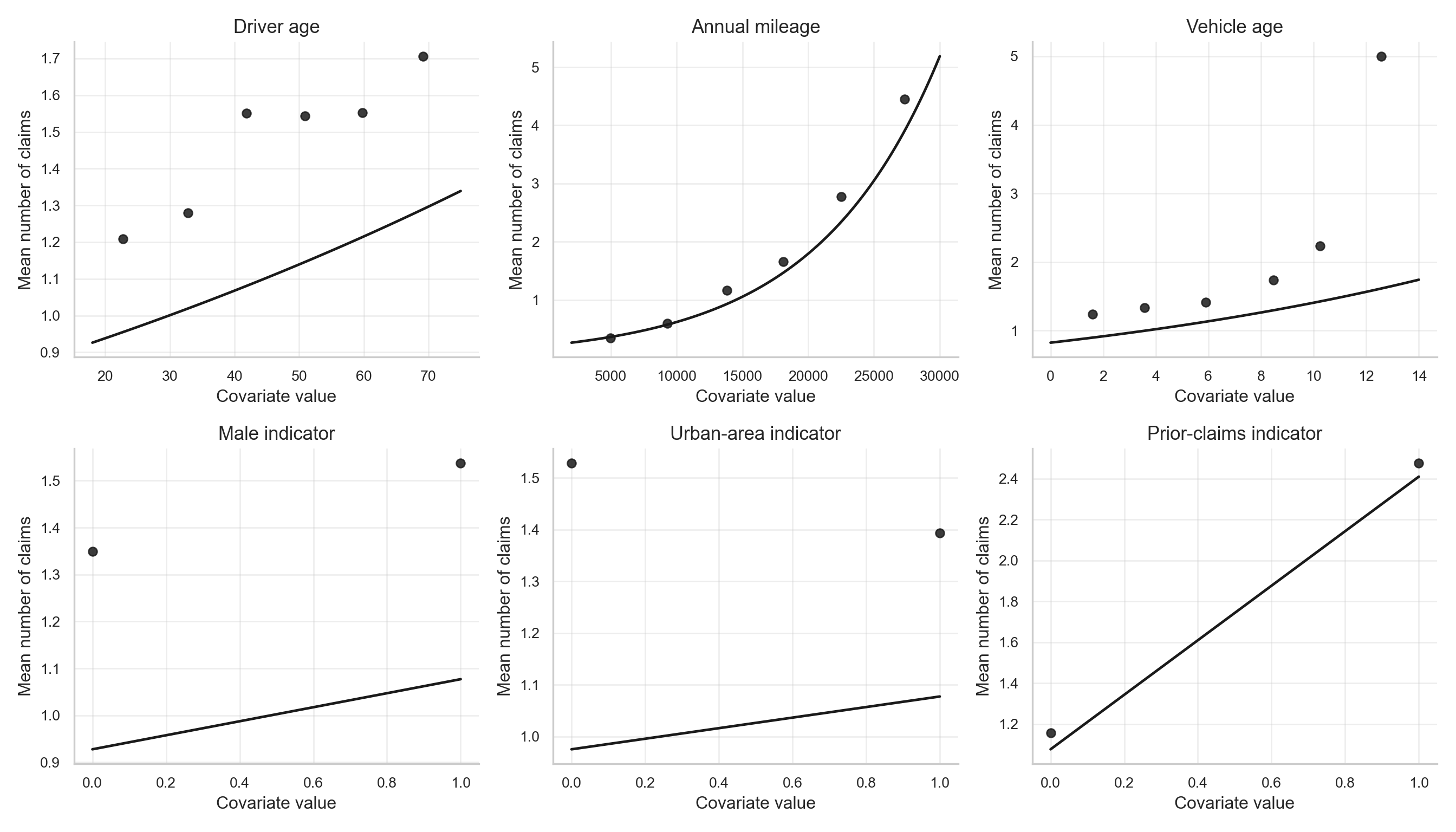
The fitted patterns in Figure 12.10 show why the Poisson baseline is informative. The fitted mean count increases from about 0.2656 to about 5.188 across the mileage range, and from about 0.8247 to about 1.742 across the vehicle-age range, with other covariates held at typical training-set values. The prior-claims panel also shows a clear fitted increase, from about 1.077 to about 2.41.
Classical Poisson Regression therefore preserves the count response and gives a direct model for claim frequency. The fitted patterns in Figure 12.10 and Figure 12.11 are useful because they show the same directional signals already suggested by the EDA: mileage, prior claims, and vehicle age are associated with higher expected counts. At the same time, the fitted Poisson curves are pulled toward the many zero observations. In practical terms, this means that a one-process Poisson model can follow the broad trend but still understate the expected count in parts of the covariate range where the empirical mean is high, such as the upper annual-mileage bins. The model is trying to represent both the zero pile-up and the positive-count pattern with one mean function, so the excess zeros can pull the fitted mean downward.
This is the key limitation for the present chapter. If many zeros arise from a separate mechanism, a single Poisson mean may have difficulty representing both the large mass at zero and the positive-count distribution. The next check makes this limitation explicit by comparing the observed zero frequency with the zero frequency implied by the fitted Poisson means.
The calculation is straightforward once the fitted Poisson means are available. For each policyholder, the fitted Classical Poisson Regression model gives a fitted mean \(\widehat{\lambda}_i\). Under the Poisson model, the probability of observing zero claims for that same policyholder is \(\exp(-\widehat{\lambda}_i)\). Averaging these fitted zero probabilities gives the model-implied zero rate; summing them gives the expected number of zero-claim policyholders under the fitted Poisson model.
# Step 1: extract the fitted Poisson means for the training rows.
cpr_fitted_mu_r <- predict(cpr_model_r, type = "response")

# Step 2: convert each fitted mean into its implied zero probability.
cpr_fitted_zero_prob_r <- exp(-cpr_fitted_mu_r)

# Step 3: compare the observed and model-implied zero frequencies.
cpr_zero_check_r <- tibble(
  Summary = c(
    "Observed zero rate",
    "Average fitted Poisson zero probability",
    "Observed minus fitted zero rate",
    "Observed number of zeros",
    "Expected number of zeros under fitted Poisson"
  ),
  Value = c(
    mean(train_data$claims == 0, na.rm = TRUE),
    mean(cpr_fitted_zero_prob_r, na.rm = TRUE),
    mean(train_data$claims == 0, na.rm = TRUE) -
      mean(cpr_fitted_zero_prob_r, na.rm = TRUE),
    sum(train_data$claims == 0, na.rm = TRUE),
    sum(cpr_fitted_zero_prob_r, na.rm = TRUE)
  )
)

cpr_zero_check_r |>
  fmt_table() |>
    print_as_dt()
# Step 1: recreate the design matrix used by the fitted Poisson model.
X_cpr = sm.add_constant(
training_data[zip_model_covariates_py].astype(float),
has_constant="add"
)
# Step 2: extract the fitted Poisson means for the training rows.
cpr_fitted_mu_py = cpr_model_py.predict(X_cpr)
# Step 3: convert each fitted mean into its implied zero probability.
cpr_fitted_zero_prob_py = np.exp(-cpr_fitted_mu_py)
# Step 4: compare the observed and model-implied zero frequencies.
observed_zero_rate_py = (training_data["claims"] == 0).mean()
observed_zero_n_py = int((training_data["claims"] == 0).sum())
cpr_zero_check_py = pd.DataFrame({
"Summary": [
"Observed zero rate",
"Average fitted Poisson zero probability",
"Observed minus fitted zero rate",
"Observed number of zeros",
"Expected number of zeros under fitted Poisson",
],
"Value": [
observed_zero_rate_py,
cpr_fitted_zero_prob_py.mean(),
observed_zero_rate_py - cpr_fitted_zero_prob_py.mean(),
observed_zero_n_py,
cpr_fitted_zero_prob_py.sum(),
],
})In Table 12.27 and Table 12.28, the observed zero rate is 51%, while the average zero probability implied by the fitted Classical Poisson model is about 32.87%. The gap is about 18.13%, or roughly 408 observed zeros versus 262.9 expected zeros under the fitted Poisson means. This does not mean the Poisson model is useless; it captures important count-scale gradients. It does mean that the model has no separate mechanism for the extra zeros, and that the same fitted mean must compromise between explaining zero observations and positive counts.
12.6.3 Why ZIP can be useful here
The two simpler approaches highlight the motivation for ZIP regression.
| Approach | Response Used | What the fitted comparison shows here | Main Limitation in This Example |
|---|---|---|---|
| Binary Logistic Regression |
\(H_i = \mathbb{I}(Y_i > 0)\), implemented as has_claim
|
Table 12.21 and Figure 12.8 show a strong zero-versus-nonzero signal for annual_mileage and prior_claims; the fitted odds ratios are about 5.448 and 4.672 for the scaled comparisons. |
It collapses all positive counts into one category. In the training data, positive counts average 2.957 and can reach 14, so a binary response discards meaningful claim-frequency information. |
| Classical Poisson Regression |
\(Y_i\), implemented as claims
|
Table 12.25 and Figure 12.10 show clear count-scale gradients, especially for annual_mileage, prior_claims, and vehicle_age; their scaled fitted rate ratios are about 2.889, 2.237, and 1.306. |
It assumes a single Poisson count-generating process. As shown in Table 12.27 and Table 12.28, its fitted zero probability is about 32.87%, below the observed zero rate of 51%. The excess zeros also pull the fitted count curve downward, which can understate the empirical mean count in high-risk regions of the covariate space. |
| Zero-Inflated Poisson Regression |
\(Y_i\), implemented as claims
|
The EDA and the two baseline fits point to two simultaneous features: a strong zero-versus-nonzero process and meaningful variation in the positive count scale. | It is more complex, so it should be used when the EDA and subject-matter context justify a separate zero-generating mechanism. |
In the insurance-claims setting, the EDA suggested a large zero-claim group and a positive-count pattern among the remaining observations. Logistic Regression describes the first piece: who is likely to file at least one claim. Classical Poisson Regression describes the second piece: how expected claim counts change with the covariates, but it has to use the same mean structure to explain both the many zeros and the positive-count trend. ZIP regression is useful because it gives these two pieces separate but connected roles. One component models extra zeros, while the other models claim counts among observations that remain in the count-generating process.
12.7 Data Modelling
The previous section used Binary Logistic Regression and Classical Poisson Regression as baseline comparisons. We now define the model that this chapter is actually about: Zero-Inflated Poisson Regression. The goal of this section is to move from the empirical motivation to the formal modelling equations that will later be estimated in R and Python.
We first describe the model generically, without attaching the covariates to the insurance example. After that, we translate the notation back to the variables defined in Table 12.18.
12.7.1 Response distribution: a zero-inflated Poisson random variable
Let \(Y_i\) be a nonnegative count response for observational unit \(i\), where \(i = 1, 2, 3, \ldots, n\), and \(n\) is the number of observations. A Zero-Inflated Poisson model assumes that each observation can arise from one of two latent states:
- A structural-zero state, where the response is forced to be zero.
- A count-generating state, where the response follows an ordinary Poisson distribution and can still equal zero by chance.
To represent this idea, let’s define a latent indicator \(S_i\) which will work as an auxiliary variable to represent the presence of a structural zero. We have then that \(S_i = 1\) means that observation \(i\) belongs to the structural-zero state, and \(S_i = 0\) means that observation \(i\) belongs to the Poisson count-generating state. Let
\[ S_i \sim \operatorname{Bernoulli}(\pi_i), \tag{12.10}\]
where \(\pi_i = P(S_i = 1)\) is the probability that observation \(i\) belongs to the structural-zero state. Conditional on this latent state, the response is generated as follows:
\[ Y_i \mid S_i = \begin{cases} 0, & \text{if } S_i = 1, \\ \operatorname{Poisson}(\lambda_i), & \text{if } S_i = 0. \end{cases} \tag{12.11}\]
The parameter \(\lambda_i > 0\) is the Poisson mean in the count-generating state. The structural-zero state is important because it adds zeros that cannot be explained by the ordinary Poisson process alone. In other words, some zeros are structural zeros, while other zeros are ordinary sampling zeros generated by the Poisson distribution.
Using Equation 12.10 and Equation 12.11, the probability of observing zero can be built by separating the two latent states. The event \(Y_i = 0\) can happen in two ways:
- the observation belongs to the structural-zero state, or
- the observation belongs to the count-generating state and the Poisson random variable happens to equal zero.
The law of total probability gives
\[ \begin{aligned} P(Y_i = 0) &= P(Y_i = 0, S_i = 1) + P(Y_i = 0, S_i = 0) \\[6pt] &= \underbrace{P(S_i = 1)}_{\substack{\text{structural-zero} \\ \text{state}}} + \underbrace{P(S_i = 0)}_{\substack{\text{count-generating} \\ \text{state}}} \underbrace{P(Y_i = 0 \mid S_i = 0)}_{\substack{\text{ordinary Poisson} \\ \text{zero}}} \\[6pt] &= \underbrace{\pi_i}_{\substack{\text{extra-zero} \\ \text{probability}}} + \underbrace{(1 - \pi_i)}_{\substack{\text{probability of being} \\ \text{in the count state}}} \quad \cdot \quad \underbrace{\exp(-\lambda_i)}_{\substack{\text{Poisson probability} \\ \text{of zero}}} \\[6pt] &= \pi_i + (1 - \pi_i)\exp(-\lambda_i). \end{aligned} \tag{12.12}\]
The first term is the extra mass placed at zero by the structural-zero state. The second term is the ordinary Poisson zero probability, but it is weighted by \(1 - \pi_i\) because it can occur only among observations in the count-generating state.
For a positive count \(y_i = 1, 2, 3, \ldots\), the structural-zero state cannot produce the observed value. Therefore, the only contributing path is the count-generating state followed by a Poisson draw equal to \(y_i\):
\[ \begin{aligned} P(Y_i = y_i) &= P(Y_i = y_i, S_i = 1) + P(Y_i = y_i, S_i = 0) \\[6pt] &= \underbrace{P(S_i = 1)P(Y_i = y_i \mid S_i = 1)}_{\substack{=\,0 \\ \text{structural-zero state cannot} \\ \text{produce a positive count}}} + \underbrace{P(S_i = 0)}_{\substack{\text{count-generating} \\ \text{state}}} \underbrace{P(Y_i = y_i \mid S_i = 0)}_{\substack{\text{Poisson probability} \\ \text{of } y_i}} \\[6pt] &= 0 + \underbrace{(1 - \pi_i)}_{\substack{\text{probability of being} \\ \text{in the count state}}} \quad \cdot \quad \underbrace{\frac{\exp(-\lambda_i)\lambda_i^{y_i}}{y_i!}}_{\substack{\text{Poisson PMF} \\ \text{at } y_i}} \\[6pt] &= (1 - \pi_i)\frac{\exp(-\lambda_i)\lambda_i^{y_i}}{y_i!}, \qquad y_i = 1, 2, 3, \ldots \end{aligned} \tag{12.13}\]
Equations Equation 12.12 and Equation 12.13 define the Zero-Inflated Poisson probability model.
More formally, this distribution is represented as the following Probability Mass Function (PMF):
\[ P(Y_i=y_i)= \begin{cases} \pi_i+(1-\pi_i)\exp(-\lambda_i), & \text{if } y_i = 0 \\[6pt] (1-\pi_i)\dfrac{\exp(-\lambda_i) \lambda_i^{y_i}}{y_i!}, & \text{if } y_i = 1, 2, 3 \dots \end{cases} \tag{12.14}\]
This also shows why the ZIP model can produce more zeros than an ordinary Poisson model: the zero probability is not only \(\exp(-\lambda_i)\), but \(\pi_i + (1 - \pi_i)\exp(-\lambda_i)\).
The conditional mean under this model is
\[ \mathbb{E}(Y_i) = \sum_{y_i=0}^\infty y_i P(Y_i=y_i) = (1 - \pi_i)\lambda_i. \tag{12.15}\]
Thus, the expected count depends on both components. A larger \(\lambda_i\) increases the expected count among observations in the count-generating state, while a larger \(\pi_i\) lowers the marginal expected count by moving more observations into the structural-zero state.
Tip on deriving the expected value of a ZIP random variable
A convenient way to derive the expected value of a Zero-Inflated Poisson random variable is to start directly from its PMF and then notice that the zero term contributes nothing to the expectation.
Suppose that, for policyholder \(i\),
\[ P(Y_i = y_i) = \begin{cases} \pi_i + (1 - \pi_i)\exp(-\lambda_i), & y_i = 0, \\[6pt] (1 - \pi_i)\dfrac{\exp(-\lambda_i)\lambda_i^{y_i}}{y_i!}, & y_i = 1, 2, 3, \ldots \end{cases} \]
where \(\pi_i\) is the probability of belonging to the structural-zero state, and \(\lambda_i\) is the Poisson mean in the count-generating state.
The expectation is
\[ \mathbb{E}(Y_i) = \sum_{y_i = 0}^{\infty} y_i P(Y_i = y_i). \]
The first term of this sum corresponds to \(y_i = 0\). Since it is multiplied by zero, it drops out:
\[ \mathbb{E}(Y_i) = \sum_{y_i = 1}^{\infty} y_i (1 - \pi_i) \dfrac{\exp(-\lambda_i)\lambda_i^{y_i}}{y_i!}. \]
Now factor out the terms that do not depend on \(y_i\):
\[ \mathbb{E}(Y_i) = (1 - \pi_i)\exp(-\lambda_i) \sum_{y_i = 1}^{\infty} \dfrac{y_i\lambda_i^{y_i}}{y_i!}. \]
Since
\[ \dfrac{y_i}{y_i!} = \dfrac{1}{(y_i - 1)!}, \]
we can rewrite the sum as
\[ \mathbb{E}(Y_i) = (1 - \pi_i)\exp(-\lambda_i) \sum_{y_i = 1}^{\infty} \dfrac{\lambda_i^{y_i}}{(y_i - 1)!}. \]
Now change the index by letting \(p = y_i - 1\). When \(y_i = 1\), \(p = 0\), so
\[ \mathbb{E}(Y_i) = (1 - \pi_i)\exp(-\lambda_i) \sum_{p = 0}^{\infty} \dfrac{\lambda_i^{p + 1}}{p!}. \]
Factor out one \(\lambda_i\) from \(\lambda_i^{p+1}\):
\[ \mathbb{E}(Y_i \mid \mathbf{x}_i) = (1 - \pi_i)\exp(-\lambda_i) \sum_{p = 0}^{\infty} \dfrac{\lambda_i^{p}\lambda_i}{p!} = (1 - \pi_i)\exp(-\lambda_i)\lambda_i \sum_{p = 0}^{\infty} \dfrac{\lambda_i^p}{p!}. \]
Finally, recall the exponential McLaurin series expansion
\[ \exp(x) = \sum_{n = 0}^{\infty} \dfrac{x^n}{n!} \] where \(x\) is equivalent to \(\lambda_i\), and \(n\) is equivalent to \(p\).
Therefore,
\[ \mathbb{E}(Y_i) = (1 - \pi_i)\exp(-\lambda_i)\lambda_i\exp(\lambda_i) = (1 - \pi_i)\exp(-\lambda_i + \lambda_i) \cdot \lambda_i = (1 - \pi_i)\lambda_i. \]
So, for a ZIP model,
\[ \boxed{ \mathbb{E}(Y_i) = (1 - \pi_i)\lambda_i } \]
This result is intuitive: the count-generating Poisson process has mean \(\lambda_i\), but it is active only with probability \(1 - \pi_i\). The structural-zero group contributes no counts to the expectation.
12.7.2 Modelling the parameters with covariates
Now suppose that each observational unit has \(k\) candidate covariates. A compact covariate vector can be written as
\[ \mathbf{x}_i = (1, x_{1,i}, x_{2,i}, \ldots, x_{k,i})^\top, \tag{12.16}\]
The main implication of combining a structural-zero state with a count-generating state is that the model has two systematic components instead of one. One component describes the structural-zero probability \(\pi_i\) from Equation 12.10, and the other describes the Poisson mean \(\lambda_i\) from Equation 12.11. This is the main difference from the single-component GLM examples introduced earlier in the cookbook.
For this chapter, we use \(\alpha\) coefficients for the structural-zero component and \(\beta\) coefficients for the count component.
The structural-zero probability is modelled with a logit link:
\[ \operatorname{logit}(\pi_i) = \log\left(\frac{\pi_i}{1 - \pi_i}\right) = \alpha_0 + \alpha_1x_{1,i} + \alpha_2x_{2,i} + \cdots + \alpha_kx_{k,i}. \tag{12.17}\]
The fraction inside the logarithm,
\[ \frac{\pi_i}{1 - \pi_i}, \]
is an odds. In this ZIP setting, it compares the probability of belonging to the structural-zero state, \(\pi_i\), with the probability of not belonging to that state, \(1 - \pi_i\). In other words, the logit link models the log of the ratio
\[ \frac{\text{probability of structural-zero membership}}{\text{probability of count-generating membership}}. \]
The right-hand side of Equation 12.17 is the linear systematic component. It is called linear because the coefficients enter additively on the link-function scale: an intercept plus one coefficient-weighted contribution from each covariate. The model is not claiming that \(\pi_i\) itself is a linear function of the covariates. Instead, it claims that the log-odds of structural-zero membership are linear in the covariates.
Alternatively we can also define the \(\boldsymbol{\alpha}\) vector as
\[ \boldsymbol{\alpha} = (\alpha_0, \alpha_{1}, \alpha_{2}, \ldots, \alpha_{k})^\top, \tag{12.18}\]
and in matrix-vector product form, the same equation is
\[ \operatorname{logit}(\pi_i) = \mathbf{x}_i^\top \boldsymbol{\alpha}. \tag{12.19}\]
Equivalently,
\[ \pi_i = \frac{\exp(\mathbf{x}_i^\top \boldsymbol{\alpha})}{1 + \exp(\mathbf{x}_i^\top \boldsymbol{\alpha})}. \tag{12.20}\]
A positive \(\alpha_j\) means that larger values of \(x_{j,i}\) are associated with higher log-odds of belonging to the structural-zero state, holding the other covariates fixed. On the exponential scale, \(\exp(\alpha_j)\) is an odds ratio for structural-zero membership. The exact interpretation depends on the type of covariate:
- If \(x_{j,i}\) is continuous, then \(\alpha_j\) is the change in the log-odds of structural-zero membership for a one-unit increase in that covariate, holding all other covariates fixed. In practice, the one-unit change should be chosen carefully. For example, a one-kilometre change in annual mileage may be too small to communicate clearly, so a later interpretation may use \(10{,}000\alpha_j\) and \(\exp(10{,}000\alpha_j)\) instead.
- If \(x_{j,i}\) is an ordered discrete or integer-valued covariate, then \(\alpha_j\) is still interpreted as a one-unit increase, but the unit has the meaning of the variable. For example, if vehicle age is measured in years, then \(\alpha_j\) is the change in log-odds associated with one additional year of vehicle age, holding the other covariates fixed.
- If \(x_{j,i}\) is a binary indicator, then \(\alpha_j\) compares the group coded \(1\) with the group coded \(0\). For example, if
prior_claimsis coded as \(1\) for prior claims and \(0\) for no prior claims, then \(\exp(\alpha_j)\) is the structural-zero odds ratio for policyholders with prior claims relative to policyholders without prior claims, holding the other covariates fixed. - If \(x_{j,i}\) represents a nominal categorical variable with more than two categories, the interpretation depends on the dummy or indicator coding. Each coefficient compares one category with the reference category, not with a one-unit numerical increase. For instance, if vehicle type had categories such as
sedan,SUV, andtruck, andsedanwere the reference category, then theSUVcoefficient would compare SUVs with sedans, holding the other covariates fixed.
The Poisson count mean is modelled with a log link:
\[ \log(\lambda_i) = \beta_0 + \beta_1x_{1,i} + \beta_2x_{2,i} + \cdots + \beta_mx_{m,i}. \tag{12.21}\]
The log link plays a similar role for the count-generating mean. The left-hand side, \(\log(\lambda_i)\), is the logarithm of the Poisson mean among observations that remain in the count-generating state. The right-hand side is another linear systematic component: an intercept plus coefficient-weighted covariate contributions. This means that the model is linear on the log-mean scale, while \(\lambda_i\) itself remains positive after applying the inverse link in Equation 12.24.
Alternatively we can also define the \(\boldsymbol{\beta}\) vector as
\[ \boldsymbol{\beta} = (\beta_0, \beta_{1}, \beta_{2}, \ldots, \beta_{k})^\top, \tag{12.22}\]
and in matrix-vector product form, the same equation is
\[ \log(\lambda_i) = \mathbf{x}_i^\top \boldsymbol{\beta}. \tag{12.23}\]
Equivalently,
\[ \lambda_i = \exp(\mathbf{x}_i^\top \boldsymbol{\beta}). \tag{12.24}\]
A positive \(\beta_j\) means that larger values of \(x_{j,i}\) are associated with a higher log mean in the Poisson count-generating state, holding the other covariates fixed. On the exponential scale, \(\exp(\beta_j)\) is a rate ratio for the Poisson mean among observations that remain in the count-generating state. As with the \(\alpha\) coefficients, the exact interpretation depends on the type of covariate:
- If \(x_{j,i}\) is continuous, then \(\beta_j\) is the change in the log mean count for a one-unit increase in the covariate, holding the other covariates fixed. The rate ratio for a larger change \(c\) is \(\exp(c\beta_j)\).
- If \(x_{j,i}\) is an ordered discrete or integer-valued covariate, then \(\beta_j\) is the change in the log mean count for one additional unit of that variable. For example, if vehicle age is measured in years, then \(\exp(\beta_j)\) is the fitted multiplicative change in the count-generating mean for one additional year of vehicle age.
- If \(x_{j,i}\) is a binary indicator, then \(\exp(\beta_j)\) compares the fitted count-generating mean for the group coded \(1\) with the group coded \(0\), holding the other covariates fixed.
- If \(x_{j,i}\) represents a nominal categorical variable with more than two categories, each dummy-variable coefficient compares that category with the reference category. The coefficient should not be read as a numerical one-unit increase through the category labels.
In the current insurance-claims dataset, the available categorical variables are binary indicators. However, this nominal-categorical distinction is important for future applications of ZIP regression where variables such as region, policy type, vehicle class, or occupation group may enter the model.
Putting both components together shows how the two link functions determine the marginal mean of the observed count response. The count component contributes \(\lambda_i = \exp(\mathbf{x}_i^\top\boldsymbol{\beta})\), while the zero-inflation component contributes the probability of not being in the structural-zero state, \(1 - \pi_i\). Therefore, using Equation 12.15, Equation 12.20, and Equation 12.24, the overall mean can be written as follows:
\[ \begin{aligned} \mathbb{E}(Y_i \mid \mathbf{x}_i) &= (1-\pi_i)\lambda_i \\[10pt] &= \bigg(1-\frac{\exp(\mathbf{x}_i^\top \boldsymbol{\alpha})}{1 + \exp(\mathbf{x}_i^\top \boldsymbol{\alpha})}\bigg)\cdot \exp(\mathbf{x}_i^\top \boldsymbol{\beta})\\[10pt] &=\bigg(\frac{1}{1+\exp(\mathbf{x}_i^\top \boldsymbol{\alpha})} \bigg)\cdot \exp(\mathbf{x}_i^\top \boldsymbol{\beta})\\[10pt] &=\frac{\exp(\mathbf{x}_i^\top \boldsymbol{\beta})}{1+\exp(\mathbf{x}_i^\top \boldsymbol{\alpha})}\\[10pt] &=\dfrac{\exp(\beta_0+\beta_1 x_{1,i} + \beta_2 x_{2,i} + \dots +\beta_k x_{k,i})}{1+\exp(\alpha_0+\alpha_1 x_{1,i} + \alpha_2 x_{2,i} + \dots +\alpha_k x_{k,i})} \end{aligned} \tag{12.25}\]
Heads-up on using the same covariates in both components!
The notation above uses the same covariate vector \(\mathbf{x}_i\) in both components for simplicity and for consistency with the running example. In practice, the zero-inflation component and the count component can use different covariate sets. For example, one component could use all candidate regressors, while the other uses a smaller subset selected for substantive reasons: nature of the problem, feature selection, reducing model complexity, etc.
12.7.3 Assumptions behind the ZIP formulation
The ZIP model is useful only when its two-component story is plausible. In this chapter, the main assumptions are:
Count response: The response \(Y_i\) is a nonnegative integer-valued count. This is the scale assumed by the ZIP PMF in Equation 12.14. In the running example,
claimssatisfies this requirement because it records \(0, 1, 2, \ldots\) claims.Independent observations: Conditional on the covariates and model parameters, observations are treated as independent. In practical terms, the model is not explicitly accounting for repeated measurements on the same policyholder, household clustering, geographic clustering, or time-series dependence. If those structures exist, the basic ZIP model may need to be extended.
Two zero sources: It is substantively plausible that some zeros are structural zeros, while other zeros arise from the Poisson count-generating process. This is the distinction encoded by \(S_i\) in Equation 12.10 and Equation 12.11. Without a credible two-source explanation for zeros, the extra zero component may be difficult to justify.
Correct component interpretation: The zero-inflation component models \(\pi_i\), the probability of belonging to the structural-zero state. The count component models \(\lambda_i\), the Poisson mean among observations that remain in the count-generating state. These are not interchangeable. A covariate in the \(\alpha\) component changes the structural-zero mechanism; a covariate in the \(\beta\) component changes the count-generating mean.
Link-function structure: The logit link in Equation 12.17 is assumed to be a reasonable way to connect covariates to \(\pi_i\), and the log link in Equation 12.21 is assumed to be a reasonable way to connect covariates to \(\lambda_i\). This means the model is additive and linear on the link scales, not necessarily on the original probability or mean scales.
Poisson count-generating state: Conditional on being in the count-generating state, the Poisson mean-variance relationship is a reasonable starting point. The ZIP model adds extra zeros, but it does not by itself solve every kind of overdispersion in the positive-count process.
Enough information for two components: There are enough positive counts, enough zeros, and enough covariate variation to estimate both the \(\alpha\) and \(\beta\) components without severe instability. Because both components are estimated at the same time, sparse data or weakly separated groups can make the two sets of coefficients difficult to identify precisely.
If the count-generating part is still strongly overdispersed after accounting for excess zeros, then a Zero-Inflated Negative Binomial model may be a more appropriate extension. If there is no substantive reason to distinguish structural zeros from ordinary sampling zeros, then a simpler count model may be easier to justify and communicate.
Heads-up on severe instability in ZIP models
In this context, severe instability means that the two-component ZIP model does not have enough information to estimate the structural-zero and count-generating mechanisms reliably. Symptoms may include convergence warnings, extremely large coefficient estimates, very wide standard errors, fitted probabilities very close to \(0\) or \(1\), or coefficient estimates that change dramatically after small changes to the data or covariate set.
This matters because the ZIP model estimates both \(\boldsymbol{\alpha}\) and \(\boldsymbol{\beta}\). If the data contain many zeros but very few positive counts, the model may struggle to decide whether a covariate belongs mainly in the structural-zero story, the count-generating story, or both. In those cases, coefficient tables should be interpreted cautiously, and predicted probabilities, fitted means, sensitivity checks, or simpler comparison models may be more informative.
Tip on Bayesian extensions for limited data
The ZIP model has a naturally hierarchical interpretation: an observation first belongs either to a structural-zero state or to a count-generating state, and then the count-generating state follows a Poisson model. When the dataset is limited, this two-component structure can make the fitted coefficients and their standard errors sensitive to small changes in the data.
A Bayesian version of ZIP regression can sometimes help in this situation by placing prior distributions on the \(\alpha\) and \(\beta\) coefficients. If those priors are sufficiently informative, relevant to the problem context, and carefully justified, they can regularize unstable estimates and make the uncertainty in both components more explicit.
That said, a Bayesian ZIP model is not automatically better. Weak or poorly chosen priors may not solve the instability problem, and overly strong priors can dominate the data. Bayesian ZIP regression is therefore a useful extension to know about, especially when data are sparse, but exploring it in detail is outside the scope of this chapter and outside the main purpose of this cookbook.
12.7.4 Interpretation caveats
This can produce results that feel counter-intuitive at first. For example, a covariate could have a positive \(\alpha_j\) and a positive \(\beta_j\). In that case, higher values of the covariate are associated with higher odds of being in the structural-zero state, but also with a higher expected count among observations that are not structural zeros. These statements are not contradictory because they refer to different latent parts of the model.
An example could be a public-health outreach programme. Suppose the response is the number of emergency department visits in a year, and one covariate indicates whether a person is enrolled in an intensive care-management programme. Enrollment might have a positive zero-inflation coefficient if many enrolled people are stable, closely monitored, and therefore unlikely to visit the emergency department at all. At the same time, enrollment might have a positive count-component coefficient because, among the enrolled people who are not in the structural-zero group, many are high-need patients who can have repeated emergency visits. The same covariate can therefore point toward more zeros in one latent subgroup and larger counts in the remaining at-risk subgroup.
A concrete insurance example, using a covariate not present in the current dataset, is enrollment in a dash-cam-based safe-driving programme. Such a programme could be associated with higher odds of structural-zero membership if many enrolled drivers are cautious drivers who rarely file claims. However, among enrolled drivers who are still in the count-generating state, claim counts could be higher if the programme is especially attractive to high-exposure drivers, fleet drivers, or drivers who report minor incidents more consistently because the dash-cam system records them. In that case, the zero-inflation coefficient and the count-component coefficient could both be positive without implying a contradiction.
The marginal expected count in Equation 12.15 depends on both \(\pi_i\) and \(\lambda_i\). Therefore, a coefficient in one component should not automatically be interpreted as the total effect of a covariate on the observed count. For a continuous covariate that appears in both components, the marginal mean combines the two linear predictors through Equation 12.25, so the direction of the overall fitted mean can depend on both \(\alpha_j\) and \(\beta_j\), as well as on the current value of \(\pi_i\).
Tip on reading ZIP coefficients
A positive count-component coefficient and a positive zero-inflation coefficient do not mean the model is wrong. They may indicate a population where a covariate separates two kinds of observations: a subgroup increasingly likely to have no events at all, and a remaining at-risk subgroup with larger expected counts. This is one reason predicted probabilities, fitted means, and marginal effects are often more intuitive than coefficient tables alone.
12.7.5 ZIP model for the insurance-claims running example
We now return to the notation from Table 12.18. For policyholder \(i\), the response is \(Y_i = \texttt{claims}_i\), and the six candidate covariates are
\[ \mathbf{x}_i = \left(1, x_{1,i}, x_{2,i}, x_{3,i}, x_{4,i}, x_{5,i}, x_{6,i}\right)^\top, \tag{12.26}\]
where \(x_{1,i}\) is driver_age, \(x_{2,i}\) is annual_mileage, \(x_{3,i}\) is vehicle_age, \(x_{4,i}\) is male, \(x_{5,i}\) is urban_area, and \(x_{6,i}\) is prior_claims.
For the zero-inflation component, we write
\[ \log\left(\frac{\pi_i}{1 - \pi_i}\right) = \alpha_0 + \alpha_1x_{1,i} + \alpha_2x_{2,i} + \alpha_3x_{3,i} + \alpha_4x_{4,i} + \alpha_5x_{5,i} + \alpha_6x_{6,i}. \tag{12.27}\]
Here, \(\pi_i\) is the probability that policyholder \(i\) belongs to the structural-zero group. For example, \(\alpha_2\) describes how annual mileage is associated with the log-odds of being in that structural-zero group, holding the other covariates fixed.
For the count component, we write
\[ \log(\lambda_i) = \beta_0 + \beta_1x_{1,i} + \beta_2x_{2,i} + \beta_3x_{3,i} + \beta_4x_{4,i} + \beta_5x_{5,i} + \beta_6x_{6,i}. \tag{12.28}\]
Here, \(\lambda_i\) is the expected number of claims for policyholder \(i\) conditional on being in the count-generating state. For example, \(\beta_2\) describes how annual mileage is associated with the log mean claim count among policyholders who remain in the count-generating process, holding the other covariates fixed.
Together, Equation 12.27 and Equation 12.28 define the working ZIP model for the insurance-claims example. This specification uses the same six covariates in both components, which is useful for teaching because it lets us compare how the same regressor can behave differently in the structural-zero and count-generating parts of the model.
The combination of these two would look like this for the mean response, recalling Equation 12.25:
\[ \mathbb{E}(Y_i \mid x_{1,i}, x_{2,i}, \dots, x_{6,i}) = \dfrac{\exp(\beta_0+\beta_1 x_{1,i} + \dots + \beta_6 x_{6,i})}{1 + \exp(\alpha_0+\alpha_1 x_{1,i} + \dots + \alpha_6 x_{6,i})} \tag{12.29}\]
12.8 Estimation
Coming soon…
12.9 Model Fitting
Coming soon…
12.10 Interpretation of Fitted Results
Coming soon…
12.11 Inference for Model Parameters
Coming soon…
12.12 Goodnes of Fit
Coming soon…
12.13 Prediction with the ZIP Model
Coming soon…
12.14 How does ZIP compare to Simpler Alternatives?
Coming soon…
12.15 Practical Considerations
Coming soon…
12.16 Chapter Summary
Coming soon…
12.17 Optional Appendices
Coming soon…